Fixed Image List Algorithm (FILA)A backtrack algorithm for solving tiling problems

I've designed a new backtrack algorithm for solving tiling problems that I call fixed image list algorithm (FILA). The algorithm is flexible in that it supports various ordering heuristics.1 By using a heuristic that always selects the first open cell, FILA behaves like Fletcher and de Bruijn's algorithms.2,3 If you use a heuristic that always picks the cell that has fewest fit options, it behaves like my most constrained hole (MCH) algorithm.4 A key distinguishing feature of FILA is that ordering heuristics return neither a target cell to fill, nor a target piece to place, but rather return a set of image lists that should be tried (where an image is defined as a particular translation of a particular rotation of a puzzle piece). The returned set contains one list of images for each uniquely shaped puzzle piece. Although the ordering heuristics that target cells are best suited to FILA, the interface does allow heuristics to target pieces, and is a subject for additional research.

This interface allows the heuristic to select and return a precalculated set of image lists that is customized in three different ways to radically reduce the size of the lists by eliminating most images that cannot possibly fit. First, because different lists are calculated for each cell, only images bounded by the puzzle walls are included in the lists. Second, some heuristics (like that used by Fletcher's algorithm) guarantee that cells are filled in a particular order. For such fixed selection order heuristics, FILA identifies this order during initialization and, through a procedure I call priority occupancy filtering (POF), only includes images in a list for a cell that do not conflict with cells that must already be filled. Third, a technique I call neighbor occupancy filtering (NOF) (which is similar to a technique Gerard Putter described to me in a 2011 e-mail conversation) precalculates a different set of image lists for each possible occupancy state of the adjacent neighbors of each target cell. For a 3D polycube puzzle, there are up to six adjacent neighbors (in the $-x$, $-y$, $-z$, $+x$, $+y$, and $+z$ directions), and so up to 64 different sets of image lists are precalculated for each puzzle cell. Later, when a cell is selected by the heuristic, the current occupancy state of those adjacent neighbors is determined, and the set of image lists corresponding to that compound state is returned, guaranteeing no image conflicts with those neighboring cells. In this way, the number of images that must be tried by FILA at each recursive step is radically reduced, improving algorithm efficiency relative to other algorithms that make no such optimization, but without the expense of continuous list maintenance as is required by Donald Knuth's DLX algorithm.

Version 2.0 of my polycube puzzle solver only includes the DLX and FILA algorithms, but the retired algorithms (de Bruijn, EMCH, and MCH) can all be recreated with FILA by using the f (first), e (estimate), and s (size) heuristics respectively. In addition all of the other implemented heuristics, previously only available to DLX, may now also be used with FILA. Despite the additional abstraction, the new FILA algorithm (even with the new NOF optimization disabled) has improved puzzle solve times (I've seen from 10% to 35%). Enabling NOF (by simply adding -n to the command line) consistently provides additional incremental performance gains (I've seen from 5% to 27%). Because performance gains afforded by NOF are not attributable to changes in the search tree, but rather are limited to the efficient elimination of many images that don't fit at each branch; these performance improvement percentages should not compound as puzzle size increases, but should rather be largely independent of puzzle size.

Although the examples shown here, and the polycube puzzle solver software are limited to 3D puzzles on a cubic lattice, FILA and all of it's supporting components have no such constraints and can be used to solve tiling problems in any number of dimensions on any lattice.

December 3, 2018 Edit: I changed the title of this blog entry and edited the above introduction to make it clear that FILA was not limited to 3D puzzles on a cubic lattice.

Continue reading
Posted in Uncategorized | 6 Comments

Optimal Play of the Farkle Dice Game

I sent a link to my previous blog post on the optimal play of Farkle to Professor Todd Neller, at Gettysburg College. (I thought he might be interested in it since it was largely based on his previous analysis of the simpler dice game Pig.) We ended up talking and decided to write a paper together on optimal Farkle play. Todd presented our paper at The 15th Advances in Computer Games Conference (ACG 2017), Leiden, Netherlands, July 4, 2017. Our paper was voted second place in the best paper competition.

The paper focuses on a more minimalist rule set (whereas my previous blog post solved for facebook farkle rules). The optimization equations are much simplified by using a pair of self-referential equations describing pre-roll and post-roll game states. The paper also includes a comparison of optimal play vs max-expected-score play, a mechanism allowing a human to perfectly replicate max-expected-score play, and some simple techniques you can use to win over 49% of your games against an optimal player.

As of the time of this post, the proceedings from the conference have not yet been published, but a link to our paper is provided here for your convenience:

Optimal Play of the Farkle Dice Game

There are some POV-Ray images included in the paper that graphically show the game states from which you should roll. For your viewing pleasure, I've included below links to the images in their original 16 mega-pixel detail.

Posted in Uncategorized | Leave a comment

Maximizing Win Probability in the Game of Farkle

povray six dice
Image by Matt Busche using modified povray source by Piotr Borys

Neller and Presser modeled a simple dice game called pig as a Markov Decision Process (MDP) and used value iteration to find the optimal game winning strategy1. Inspired by their approach, I've constructed a variant of an MDP which can be used to calculate the strategy that maximizes the chances of winning 2-player farkle. Due to the three consecutive farkle penalty, an unfortunate or foolish player can farkle repeatedly to achieve an arbitrarily large negative score. For this reason the number of game states is unbounded and a complete MDP model of farkle is not possible. To bound the problem, a limit on the lowest possible banked score is enforced. The calculated strategy is shown to converge exponentially to the optimal strategy as this bound on banked scores is lowered.

Each farkle turn proceeds by iteratively making a pre-roll banking decision, a (contingent) roll of the dice, and a post-roll scoring decision. I modified the classic MDP to include a secondary (post-roll) action to fit this turn model. A reward function that incentivizes winning the game is applied. A similarly modified version of value-iteration (that maximizes the value function for both the pre-roll banking decision, and the post-roll scoring decision) is then used to find an optimal farkle strategy.

With a lower bound of -2500 points for banked scores, there are 423,765,000 distinct game states and so it is not convenient to share the entire strategy in printed form. Instead, I provide some general characterizations of the strategy. For example, if both players use this same strategy, the player going first will win 53.487% of the time. I also provide samples of complete single-turn strategies for various initial banked scores. Currently, only the strategy for Facebook Farkle has been calculated, but the strategy for other scoring variants of farkle could easily be deduced using the same software.

Continue reading
Posted in Uncategorized | 13 Comments

Tracking the States of a Set of Objects by PartitionAn Introduction to the Partition Container

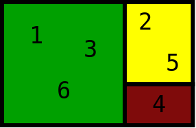
Partition of the numbers 1 through 6 into 3 groups.

In this post I share a useful programming technique I first saw used twenty-some years ago while reading through some C code. The technique combined aspects of an array and a linked-list into a single data construct. I've here abstracted the technique into a reusable container I call a partition. (If someone knows of some library in some language that offers a similar container I'd appreciate a reference.)

A partition is a high performance container that organizes a set of N sequential integer IDs (which together are called the domain) into an arbitrary number of non-overlapping groups. (I.e., each ID of the domain can be in at most one group.) The functionality of a partition includes these constant time operations:

  1. Given an ID, determine the group to which the ID belongs (if any).
  2. Given a group, find an ID in that group (if any).
  3. Given an ID, move that ID to a particular group (simultaneously removing it from the group with which it was previously a member if any).

None of the above operations use the heap and are each considerably faster than even a single push to standard implementations of a doubly linked list.

A partition has not one, but two fundamental classes: Domain and Group. The set of sequential IDs in a partition are defined by a Domain object; and a Group is a list of IDs from a Domain. Domain and Group each have two templatization parameters M and V. IDs can be bound to a user-defined member object of type M and Groups can be bound to a user defined value object of type V. Together these associations enable mappings from objects of type M (with known IDs) to objects of type V, and conversely from objects of type V (with known Groups) to a list of objects of type M.

The partition is potentially useful any time objects need to be organized into groups; and that happens all the time! In this post, I show how you can use a partition to track the states of a set of like objects. This is just one possible usage of a partition and is intended only as a tutorial example of how you can use this versatile storage class.

Continue reading
Posted in Uncategorized | Leave a comment

Solving Polyomino and Polycube Puzzles Algorithms, Software, and Solutions

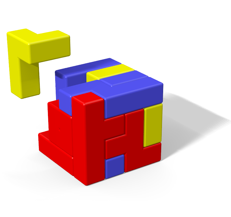
Povray image of a solution to the Tetris Cube.

Image by Matt Busche

I've implemented a set of backtrack algorithms to find solutions to various polyomino and polycube puzzles (2-D and 3-D puzzles where you have to fit pieces composed of little squares or cubes into a confined space). Examples of such puzzles include the Tetris Cube, the Bedlam Cube, the Soma Cube, and Pentominoes. My approach to the problem is perhaps unusual in that I've implemented many different algorithmic techniques simultaneously into a single puzzle solving software application. I've found that the best algorithm to use for a problem can depend on the size, and dimensionality of the puzzle. To take advantage of this, when the number of remaining pieces reaches configurable transition thresholds my software can turn off one algorithm and turn on another. Three different algorithms are implemented: de Bruijn's algorithm, Knuth's DLX, and my own algorithm which I call most-constrained-hole (MCH). DLX is most commonly used with an ordering heuristic that picks the hole or piece with fewest fit choices; but other simple ordering heuristics are shown to improve performance for some puzzles.

In addition to these three core algorithms, a set of constraints are woven into the algorithms giving great performance benefits. These include constraints on the volumes of isolated subspaces, parity (or coloring) constraints, fit constraints, and constraints to take advantage of rotational symmetries.

In this (rather long) blog entry I present the algorithms and techniques I've implemented and share my insights into where each works well, and where they don't. You can also download my software source, an executable version of the solver, and the solutions to various well known puzzles.

Continue reading
Posted in Uncategorized | 30 Comments

Matt’s Double Octagon Deck (Part 1)

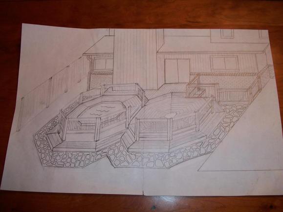
For ten years I’ve thought about replacing the decrepit deck behind my house. I wanted to do something unique to appease my sinful pride. This was the initial concept sketch for my deck consisting of two 15 foot diameter octagons placed side-by-side.

Sketch of double octagon deck

The octagon on the right is only about 14 inches above grade. The octagon on the left is one step up (maybe 7 inches higher) and surrounds an octagon-shaped hot-tub. I wanted the decking for each octagon to be laid out circularly (as shown) to emphasize the octagon shapes.

Continue reading

Posted in Uncategorized | 13 Comments

Crooked Dice in Facebook Super Farkle?

Crooked dice

I modified my Zilch strategy generation software to model the scoring rules for the Super Farkle game available at Facebook. I wasn’t previously a Facebook user so I created my account just to try out my strategy. Over several days, I played about 180 games of Farkle and was winning about 55% of the time. But I’m not sure if this means much for a few reasons.

Continue reading

Posted in Uncategorized | 5 Comments

Maximizing Expected Scores in the Game of Zilch

A Throw of the Dice
Image by Thunderchild7

Zilch is a fun little dice game codified into an online game by Gaby Vanhegan that can be played at http://playr.co.uk/. Zilch is actually a variation of the game Farkle which goes by several other names including Zonk, 5000, 10000, Wimp Out, Greed, Squelch and Hot Dice1. I've worked out the strategy that maximizes your expected game score and wanted to share the analysis, my strategy finder software, and the strategy itself. Depending on whether you have zero, one or two consecutive zilches from previous turns, three successively more conservative turn-play strategies are required to maximize your long term average score. Using these three strategies you rack up an average of 620.855 points per turn, which is the best you can possibly do.

Continue reading
Posted in Uncategorized | 18 Comments