I've designed a new backtrack algorithm for solving tiling problems that I call fixed image list algorithm (FILA). The algorithm is flexible in that it supports various ordering heuristics.1 By using a heuristic that always selects the first open cell, FILA behaves like Fletcher and de Bruijn's algorithms.2,3 If you use a heuristic that always picks the cell that has fewest fit options, it behaves like my most constrained hole (MCH) algorithm.4 A key distinguishing feature of FILA is that ordering heuristics return neither a target cell to fill, nor a target piece to place, but rather return a set of image lists that should be tried (where an image is defined as a particular translation of a particular rotation of a puzzle piece). The returned set contains one list of images for each uniquely shaped puzzle piece. Although the ordering heuristics that target cells are best suited to FILA, the interface does allow heuristics to target pieces, and is a subject for additional research.
This interface allows the heuristic to select and return a precalculated set of image lists that is customized in three different ways to radically reduce the size of the lists by eliminating most images that cannot possibly fit. First, because different lists are calculated for each cell, only images bounded by the puzzle walls are included in the lists. Second, some heuristics (like that used by Fletcher's algorithm) guarantee that cells are filled in a particular order. For such fixed selection order heuristics, FILA identifies this order during initialization and, through a procedure I call priority occupancy filtering (POF), only includes images in a list for a cell that do not conflict with cells that must already be filled. Third, a technique I call neighbor occupancy filtering (NOF) (which is similar to a technique Gerard Putter described to me in a 2011 e-mail conversation) precalculates a different set of image lists for each possible occupancy state of the adjacent neighbors of each target cell. For a 3D polycube puzzle, there are up to six adjacent neighbors (in the $-x$, $-y$, $-z$, $+x$, $+y$, and $+z$ directions), and so up to 64 different sets of image lists are precalculated for each puzzle cell. Later, when a cell is selected by the heuristic, the current occupancy state of those adjacent neighbors is determined, and the set of image lists corresponding to that compound state is returned, guaranteeing no image conflicts with those neighboring cells. In this way, the number of images that must be tried by FILA at each recursive step is radically reduced, improving algorithm efficiency relative to other algorithms that make no such optimization, but without the expense of continuous list maintenance as is required by Donald Knuth's DLX algorithm.
Version 2.0 of my polycube puzzle solver only includes the DLX and FILA algorithms, but the retired algorithms (de Bruijn, EMCH, and MCH) can all be recreated with FILA by using the f (first), e (estimate), and s (size) heuristics respectively. In addition all of the other implemented heuristics, previously only available to DLX, may now also be used with FILA. Despite the additional abstraction, the new FILA algorithm (even with the new NOF optimization disabled) has improved puzzle solve times (I've seen from 10% to 35%). Enabling NOF (by simply adding -n to the command line) consistently provides additional incremental performance gains (I've seen from 5% to 27%). Because performance gains afforded by NOF are not attributable to changes in the search tree, but rather are limited to the efficient elimination of many images that don't fit at each branch; these performance improvement percentages should not compound as puzzle size increases, but should rather be largely independent of puzzle size.
Although the examples shown here, and the polycube puzzle solver software are limited to 3D puzzles on a cubic lattice, FILA and all of it's supporting components have no such constraints and can be used to solve tiling problems in any number of dimensions on any lattice.
December 3, 2018 Edit: I changed the title of this blog entry and edited the above introduction to make it clear that FILA was not limited to 3D puzzles on a cubic lattice.
Contents
Background
I was recently invited to work on a paper on polyomino puzzle parity with professor Marcus Garvie of the University of Guelph, which got me back to the subject of polyomino and polycube puzzle solving. During my research for that paper, I read Fletcher's 1965 publication on solving the 10x6 pentomino problem shown in Figure 1, and also spent an evening making my best effort translation (via google translate) of de Bruijn's 1971/72 paper on solving the same puzzle.
Although some 50 years old, Fletcher and de Bruijn's algorithms (which are extremely similar) are still widely regarded as the fastest for many tiling problems. These algorithms define the fixed list of 63 possible rotations of the 12 pentominoes. At each recursive step, the algorithms target an unfilled cell (a hole), and attempt to fill that cell by translating each of the 63 piece images to the absolute position of the target, and then attempting to place each of those translated images to cover the target. Here an image is defined as a particular translation of a particular rotation of a particular puzzle piece. (This is a slightly looser definition than I used in my previous blog article4 in that here I allow an image to fall partially outside the boundary of the puzzle box as required by Fletcher and de Bruijn's algorithms. I'll use the term bounded image to refer to images contained wholly inside the puzzle box.) If you were to simultaneously watch animations of the Fletcher and de Bruijn algorithms placing and removing pieces from the puzzle as they search for solutions, you would find them to be almost identical. In particular, the search trees the two algorithms explore are identical. (I.e., the set of partial assemblies the two algorithms produce are identical.) Only the order in which the branches of that tree are explored differ.
Both Fletcher and de Bruijn modeled the 10x6 puzzle box so the shorter sides (dimension 6) are on the left and right, and the longer sides (dimension 10) are top-and-bottom. To eliminate rotationally redundant solutions, both Fletcher and de Bruijn started by placing the X piece in one of 7 locations in the upper left quadrant of the box. Then, starting with the top-left cell, the algorithms scan down searching for an unfilled puzzle cell. When the bottom edge of the puzzle box is reached, the scan continues at the top of the next column to the right. When an unfilled cell is found (the target), the algorithms try all 63 possible orientations of the 12 pentomino pieces to fill that target. For each such orientation one could try to place each of the five constituent cubes of the pentomino into the target, but because all cells to the left and directly above that cell are guaranteed to be previously filled, there is only one cell of each oriented piece that can possibly fit the puzzle. (For a more complete explanation, see Figure 2 of my previous blog article.4) So each algorithm need only try 63 images to fill the target. For each successfully placed image, the algorithm recurses, scanning for the next unfilled cell in order. When the list of images is exhausted at any particular target, the algorithms backtrack to the previous target and continue processing where it left off, considering each of the remaining images in the list at that cell.
The order in which the 63 images are considered at each cell do differ, but other than that the algorithms are identical if your view of them is limited to the animations. But internally, their designs significantly differ in how they process the 63 images to quickly sift through those that do not fit and identify the ones that do. The two approaches each have certain advantages and disadvantages in efficiency. It was these differences that got me thinking about how to better optimize this aspect of backtrack algorithms that rely on fixed image lists that ultimately led to my design of FILA.
During any particular recursive step, most of the images in the list of 63 images will be found to be unusable either because the image corresponds to a piece that is already used, or because it conflicts with pieces already placed on the board, or because it intersects the boundary of the puzzle box itself. Donald Knuth's dancing links (DLX) algorithm,1 in contrast, takes the different approach of maintaining dynamic image lists for each puzzle cell and for each puzzle shape, that are continuously pruned and restored during algorithm execution. At any recursive step, for each unfilled puzzle cell a perfect image list is available that includes all images that cover that cell, but only those images that still fit in the puzzle without conflict, and only images for pieces that are still available. Likewise, there is a perfect image list available for each remaining piece that includes all images of that piece that still fit in the puzzle without conflict. But for many problems the time to keep these lists updated is more than the time saved by not having to sift through images that are either no longer available or no longer fit.
Still, many other tiling problems, due to their curious geometries, are not efficiently solved with the simple Fletcher algorithm that always fills the puzzle from left-to-right. DLX's abstract data model easily supports any conceivable ordering heuristic allowing it to better solve these problems. Further, this same abstract data model allows it to be used for a wide variety of problem domains that go beyond tiling problems in Z^n space. Recognizing their performance advantages, FILA was designed to use fixed (precalculated) image lists, but also have the flexibility to be easily used with a variety of ordering heuristics.
In this article, I'll start by showing how Fletcher and de Bruijn sifted through the list of 63 pentomino images. I'll then detail FILA, and show how it's use of cell-specific image lists generated with POF and NOF image filtering attempts to capture the best aspects of both approaches and improve upon them.
Fletcher's Image Sifting Technique
Fletcher's approach to checking for image fits is interesting. Instead of checking the 63 images for conflicts independently, he explores the cells around the target cell following a predefined tree structure. The distance from the root to each leaf of this tree is length 5. There are 63 leaves on the tree, each corresponding to one of the 63 pentomino orientations. If either a filled cell or a puzzle wall is encountered while following a branch, then exploration of that branch is terminated and all images subtending that branch are efficiently skipped. For example, the first cell of the tree that is checked is directly below the target cell. If that cell is filled, then 29 images from the list of 63 are skipped and the cell to the immediate right of the target cell is then tested to see if it is filled. Each time a leaf is reached, the pentomino corresponding to that leaf is checked for availability (it may have already been used). If available, the pentomino is placed and the algorithm recurses.
I've mapped the tree Fletcher designed to an animated player shown in Figure 2. The black area to the left represents cells that were found to be previously filled, and the red cell (shown at step 0) is the first empty cell found during the search for an empty cell. In the original 10x6 pentomino problem, the tree cannot possibly be fully traversed because either the top or bottom of the puzzle would interfere, so I've increased the vertical dimension of the puzzle area so that the entire search tree can be examined. Each time a leaf of the tree is reached, I display an image counter in the top-right area of the puzzle so you can more easily keep track of where you are in the image list.
The entire tree can be explored with only 90 memory accesses, but in practice, far fewer steps are typically needed for the 6x10 pentomino problem as either the puzzle boundary or previously placed pieces will interrupt many branch explorations. Still, there are some aspects of this approach that are undesirable. First, Fletcher doesn't check to see whether a piece is even available until a leaf of the search tree is reached. 83% of the pieces placed during algorithm execution on the 10x6 pentomino puzzle are for the last 4 pieces of the puzzle, so a significant amount of time is spent checking to see if pieces that are no longer available will fit. Second, note that despite the tree structure, the occupancy state of many cells are checked multiple times. For example, you can see from the movie player, that the cell just to the right of the target cell is checked in steps 5, 9, 20, and 44. If that cell is filled, those four checks respectively eliminate 1, 4, 10, and 34 images. It would be nice if only one check of that cell was made and, if found to be occupied, all 49 of these conflicting images were eliminated at once. Unfortunately, due to the diversity of the pentomino shapes, there is no way to construct a simple exploration tree that avoids revisiting cells.
I'll make one other observation which is important to understanding the effectiveness of NOF filtering (discussed later). Because the puzzle is filled from left to right, cells further to the right of the root cell are decreasingly likely to be found occupied. Also, note that occupancies detected further from the root eliminate fewer images of the tree. So the cells nearest the root are among the most likely to be occupied, and also eliminate the most images when they are occupied.
De Bruijn's Image Sifting Technique
Like Fletcher, de Bruijn's software started by placing the X piece in one of 7 board positions. Then when trying to fill a targeted cell, de Bruijn simply linearly iterated over the remaining 62 images. But where Fletcher checked for piece availability last, de Bruijn made this check first. Here's is an excerpt of his program that I attempted to translate to English:
        refillingAttempt:   if warehouse[pieceNum[i]] = 0 then
                                 goto nextSlice;
                            for i:= step 1 until 4 do
                                if occupied[cell + relpos[slice, i]] = 1 then
                                    goto nextSlice;
                            warehouse[pieceNum[slice]] := 0;
                            occupied[cell] := 1;
                            for i:= step 1 until 4 do
                                occupied[cell + relpos[slice,i]] := 1;

                             .
                             .  //  recurse, or produce solution if this was the last piece
                             .

        nextSlice:           i := i + 1;
                             if i <= 63 then
                                 goto refillingAttempt;
As you can see, he kept the definitions for all 63 images in a two dimensional array: relpos[slice, i], where slice = 1 to 63 was what I'd call an image number, and i = 1 to 4 identifies the four cells of the pentomino shape (other than the cell occupying the target cell which is known to be open). The value of each array entry is an integer that specified the relative-position of a constituent cell of the image (slice). This number could be added to the integer cell location of the target to give the integer cell location of the ith cell of the slice. He also had an array pieceNum defined so that pieceNum[slice] mapped the image number slice back to it's prototype polyomino number (1 to 12). He had a boolean array called warehouse which tracked the availability of the 12 polyominoes. There was also a boolean array called occupied which tracked whether each puzzle cell was occupied or not.
This linear iteration over 62 images seems far less efficient than Fletcher's tree-like search over the grid space, but this approach does have the one advantage of not checking cell occupancy states for images of puzzle pieces that have already been placed. Because most of the search is done when only few pieces remain, most images in the list of 63 are skipped without checking board availability at all. Running the algorithm on the 6x10 pentomino problem, I found that on average only 3.65 pieces must be considered at each recursive step. Because each piece has on average 5.25 unique images, at each recursive step, the algorithm only checks cell availability for about 3.65 x 5.25 = 19.2 images.
The original motivation for my design of FILA was to try to somehow take advantage of Fletcher's approach of quickly eliminating many potential images from an image list due to a single puzzle cell being occupied, while simultaneously somehow quickly skipping over images for pieces that are no longer available (in the spirit of de Bruijn's algorithm).
Fixed Image List Algorithm (FILA)
We'll start by looking at the pseudo code for the main backtrack processing of FILA which will reveal it's recursive nature and the abstract interface to the ordering heuristic. The ordering heuristic is where the new and interesting stuff happens, and is explained over a few sections wherein the workings of NOF, and POF are explained.
solveFila
Assume you have a puzzle with $P$ polycube pieces that are to be used to fill some puzzle region $R$. We will not require that each piece have a unique shape, so let $\mathbb{Q}$ be the set of shapes unique under rotation from which the $P$ pieces are chosen. $\mathbb{Q}$ is a minimal set in that every shape in $\mathbb{Q}$ must be used to form at least one of the $P$ pieces. Let $Q$ be the number of unique shapes: $Q = \vert \mathbb{Q} \vert$. Identify each shape in $\mathbb{Q}$ with a number $s = 1, 2, 3, \ldots, Q$. The algorithm solveFila maintains an ordered set $S$ (e.g., an array) holding these shape numbers. Initialize $S$ by arbitrarily loading these numbers in order: $S_1 = 1, S_2 = 2, \ldots S_Q = Q$. Define $N_s$ to be the number of pieces having shape $s$. Initially $N_s > 0$ for all $s$, but each time a piece of shape $s$ is placed, the value of $N_s$ will be decremented, and when a piece of shape $s$ is removed, the value of $N_s$ will be incremented. So during algorithm execution, $N_s$ represents the number of pieces of shape $s$ that have yet to be placed. Let $V$ (volume) be the number of cells in the puzzle region $R$ that must be filled, and denote the cells themselves $c_0, c_1, c_2, \ldots c_{V-1}$. Although it's probably inappropriate for pseudo code, we'll assume that the occupancy state of the puzzle is modeled as a bitfield $o$, where bit $v$ of $o$ is one if and only if $c_v$ is occupied. The list $O$ is used as a stack of images currently placed in the puzzle and is used only for producing output when solutions are found.
solveFila invokes the function selectFila which returns a set $I$ of lists of (references to) images to be attempted to be placed in the puzzle. There is one image list $I_s \in I$ for each shape $s$. In general all lists in $I$ could contain images, but only the images in lists $I_s$ for which at least one piece of shape $s$ remains to be placed should be attempted to be placed in the puzzle. All image list sets are precalculated, but many such sets exist. The process by which an image list set is chosen by selectFila, and the exact content of each set are detailed in subsequent sections. Each image $i$ in $I_s$ has a layout field $L[i]$ which is itself a bitfield. Bit $v$ of $L[i]$ is set if and only if image $i$ occupies cell $c_v$.
solveFila takes three arguments: $p$ is the number of remaining puzzle pieces; $q$ is the number of remaining shapes; and $o$ is the current occupancy state of the puzzle region $R$. So to start things off, you invoke solveFila with parameters $p=P$, $q=Q$, and $o = 0$. Below, I use the notation $x \land y$ to represent the bit-wise and of bit fields $x$ and $y$, and $x \lor y$ to represent the bit-wise or of $x$ and $y$.
1.solveFila$(p, q, o)$2.If $p = 0$ process the solution and return.3.Set $I \leftarrow$selectFila$(p, q, o)$.4.For each $j \leftarrow 1, 2, 3, \ldots q$,5.set $s \leftarrow S_j$;6.set $N_s \leftarrow N_s - 1$;7.if $N_s = 0$,8.swap$(S_j, S_q)$,9.set $q \leftarrow q - 1$;10.for each $i$ in $I_s$,11.if $o \land L[i] = 0$,12.set $O_p \leftarrow i$;13.solveFila$(p-1, q, o \lor L[i])$;14.if $N_s = 0$,15.set $q \leftarrow q + 1$;16.swap$(S_j, S_q)$;17.set $N_s \leftarrow N_s + 1$.
So unlike Fletcher and de Bruijn's algorithms, FILA keeps track of which shapes still have unused pieces, and only considers placing images of those shapes. This information is maintained by lines 4-9 of the algorithm, and perhaps deserves some explanation. Line 4 iterates over the numbers $j$ from 1 to the number of remaining shapes $q$. Note that $j$ is not a shape number, but just a sequence number. The numbers of the available shapes are stored in the ordered list $S$ which serves as a warehouse of available shape numbers. The available shape numbers are kept in the first $q$ positions of $S$, so $s = S_j$ is an available shape number for all iterated $j$ values. While shape $s$ is under consideration (starting at line 5), the number of copies of that shape, $N_s$, is decremented (line 6). If that counter hits zero (line 7), then no more copies of that shape are available. In that case, the values of $S_j$ and $S_q$ are swapped (line 8) so that shape number $s$ is listed as the last available shape in $S$. Then the number of available shapes $q$ is decremented (line 9), so that subsequent recursive calls to solveFila will no longer see shape $s$ in the now smaller window into the warehouse $S$. After all images of shape $s$ have been tested for fit, and a recursive search for solutions has been performed for each image that does fit (lines 10-13), the shape bookkeeping operations (performed in lines 6-9) are undone (lines 14-17) to restore shape-related data to it's previous state, and the next sequence number $j$ is processed (starting again at line 4).
Puzzle boundary filtering, and POF and NOF filtering (explained in the next sections), can be so effective that it is not uncommon for an Image list $I_s$ to be empty. For this reason, a small overall performance benefit can be had by inserting a check immediately after line 5 to see if $I_s$ is empty, and if so, skip immediately to the next $j$ value, bypassing the shape bookkeeping updates, the pointless loop over the empty image list, and the subsequent undo of the shape bookkeeping.
selectFila
The function selectFila returns the set of image lists $I$ that should be tried by solveFila. The implementation will vary depending on the desired behavior of the ordering heuristic. I will give here three example implementations.
selectFila for Fixed-Order Heuristics
The first works well for any fixed-order ordering heuristic, wherein the heuristic keeps an array, $C$, of (references to) all the puzzle cells in a particular (fixed) order, and always picks the first unoccupied cell from this list as the fill target. Through an appropriate ordering of the cells in $C$, any fixed order heuristic can be realized. For example, by ordering the cells so as to minimize coordinates in $x$, $y$, $z$ priority order, Fletcher's left-to-right heuristic is produced. By sorting cells to maximize the quantity $x^2+y^2+z^2$, cells are filled radially from the outside towards the puzzle center. Assume the index into $C$ is zero-based: $C_0$, $C_1$, $\ldots$ $C_{V-1}$. Let each cell $c_v$ have a bit field $B[c_v]$ with only bit $v$ set, so that $c_v$ is occupied if and only if $B[c_v] \land o \ne 0$. As a performance optimization, this implementation of selectFila maintains a stack $M$, of the indices into $C$ of previously selected cells so that subsequent calls to selectFila don't have to start searching from the beginning of $C$ for the next unoccupied cell. $M_{P+1}$ is initialized to -1 to ensure the first invocation of selectFila starts its search for an empty cell at position $0$ in $C$.
selectFila is invoked with the same three arguments as solveFila: the number of remaining pieces $p$, the number of remaining shapes $q$, and the current puzzle occupancy state $o$. The function getImageListSet returns the appropriate set of image lists $I$ for the selected fill target $C_m$ and is detailed in the next section.
selectFila$(p, q, o)$ { Set $m \leftarrow M_{p+1} + 1$. While $o \land B[C_m] \ne 0$, set $m \leftarrow m + 1$. Set $M_p \leftarrow m$. ReturngetImageListSet$(C_m, o)$; }
selectFila for F Heuristic
For our second example, first recall that the puzzle cells $c$ are themselves numbered, $c_0$, $c_1$, $\ldots$, $c_{V-1}$. This numbering defines their bit position in the occupancy state variable $o$. If this ordering happens to be that of a desirable fixed order heuristic, you can use that natural order directly with no need for the list $C$. In my solver, I number my cells according to their numerical coordinate positions with the $x$ coordinate taking precedence over $y$, and $y$ taking precedence over $z$. But this ordering is exactly the left-to-right fill order used by Fletcher and de Bruijn's algorithms. I call this heuristic that just picks the first open cell the "F" heuristic. (Or you can think about the F standing for Fletcher if you want.) The F heuristic in my solver overrides the default selectFila implementation used by all other fixed-order heuristics with a simpler (and faster) implementation that takes advantage of the natural cell ordering. Abstractly, it looks like this:
selectFila$(p, q, o)$ { Set $v \leftarrow $lowestSetBit$(\lnot o)$. ReturngetImageListSet$(c_v, o)$. }
The operation $\lnot o$ is the binary negation of $o$ (to produce the bitfield representing the holes in the puzzles), and lowestSetBit(o) returns the number of the lowest bit in $o$ that's set (which most modern processors implement in silicon).
selectFila for E Heuristic
As a third example, consider a heuristic that picks a cell estimated to be hardest to fill by first identifying all cells that have a minimum number of open neighbor cells, and then picking the cell among that set at which a minimum number of images fit (by explicitly counting the number of fits). So it acts sort of like a poor man's S heuristic most often used by DLX. Give each cell $c$ an additional field $N[c]$ which is a bit field with up to six bits set that identify the occupancy bits of the adjacent neighbors of $c$ in the six ordinal directions: +x, +y, +z, -x, -y, and -z. If one or more of these six neighbors are non-existent (because $c$ is at the perimeter of the puzzle, and/or because the puzzle is only two-dimensional), then $N[c]$ will have fewer than six bits set. Then the number of open neighbor cells of $c$ may be found by counting the number of bits set in the quantity $N[c] \land \lnot o$. The algorithm below starts by loading the cells with a minimum number of open neighbors into the set $C$, then iterating over all cells in $C$ and using a fit counting helper function to find a cell for which a minimum number of images fit.
selectFila$(p, q, o)$ Set $h \leftarrow \lnot o$. Set $n_{min} \leftarrow \infty$. Set $C \leftarrow \emptyset$. For each bit number $v$ set in $h$, set $n \leftarrow $countBits$(N[c_v] \land h)$; if $n \le n_{min}$, if $n < n_{min}$, set $n_{min} \leftarrow n$; set $C \leftarrow \emptyset$; add $c_v \rightarrow C$. Set $f_{min} \leftarrow \infty$ For each $c$ in $C$, set $I \leftarrow $getImageListSet$(c, o)$; set $f \leftarrow $countFits$(I, q, o, f_{min})$; if $f < f_{min}$, set $f_{min} \leftarrow f$, set $I_{min} \leftarrow I$. Return $I_{min}$.countFits$(I, q, o, f_{max})$ Set $f \leftarrow 0$. For each $j \leftarrow 1, 2, 3, \ldots q$, set $s \leftarrow S_j$; for each $i$ in $I_s$, if $o \land L[i] = 0$, set $f \leftarrow f + 1$; if $f \ge f_{max}$, return $f$. Return $f$.
countBits$(x)$ returns the number of bits set in bit field $x$ (which is another operation that most modern processors implement in silicon.) Also note that countFits only counts image fits up to a supplied maximum. (Since we are only looking for the cell with the minimum fits, counting beyond the minimum found so far is unnecessary.)
getImageListSet
The function getImageListSet(c, o) returns an image list set $I$ (i.e., a set of lists of images). List $I_s$ in $I$ is a list of all images of shape $s$ that cover $c$ with the following two restrictions:
- No image in $I_s$ will conflict with an occupied adjacent neighbor cell of $c$ (where an adjacent neighbor is any of the neighbors in the six ordinal directions from $c$ that share a common side with $c$).
- If the ordering heuristic follows a fixed cell selection order (according to some predetermined prioritization among the puzzle cells), then no image in $I_s$ will conflict with any puzzle cell which must previously have been filled due to this prioritized selection order.
The first property is guaranteed by NOF. The second is guaranteed by POF.
Each ordering heuristic holds a two dimensional array, $A$, of image list sets. Each entry $A_{c,z}$ is an image list set composed specifically for cell $c$ and for the occupancy state of adjacent neighbors encoded in the index variable $z$. The number $z$ is called an image list set index (ILSI). Without explaining how an ILSI is calculated, getImageListSet looks (roughly) like this:
getImageListSet$(c, o)$ Set $z \leftarrow$getIlsi$(c, o)$. return $A_{c, z}$
So you simply calculate an ILSI $z$ for cell $c$, and then return the $z$th image list set for cell $c$ from the matrix $A$. I'm glossing over one detail here: each cell can use a different (optimized) getIlsi function. An updated (real) version of getImageListSet is given below after I've explained how the ILSI $z$ is calculated and by implication, how the associated image list set is defined.
Neighbor Occupancy Filtering (NOF) and Image List Set Indices (ILSI)
As a group the six adjacent neighbors of some cell $c$ can take on $2^6 = 64$ different compound states, and each of these states will have associated with it a different image list set. (Note that some neighbor occupancy states for some cells cannot be entered, and the associated image list sets for these states need not be populated.) We want to extract from the puzzle occupancy state $o$ just the six bits that represent the occupancy state of the six adjacent neighbors of $c$. Then we'll take those bits and repack them into a new bit field that is just 6 bits long. This six-bit bit field is our ILSI.
The ILSI is constructed as follows. The highest order bit of an ILSI (bit 5) is always loaded with the bit representing the occupancy state of the adjacent neighbor in the $-x$ direction relative to cell $c$. Similarly bits 4, 3, 2, 1, and 0 respectively are loaded with the bit representing the occupancy state of the adjacent neighbors in the $-y$, $-z$, $+x$, $+y$, and $+z$ directions. These assignments of neighbors to bit-positions in the ILSI are arbitrary, but must be consistent. If one or more of the six neighbors of $c$ are outside the puzzle bounds (and therefore are not represented by any bit in $o$), then a 1 is loaded into the corresponding bits in the ILSI (so that a zero consistently identifies an open neighbor).
This resulting six-bit bit field is then interpreted as an integer between 0 and 63, which is in turn used as the second index into the matrix $A$ to retrieve an image list set that contains all puzzle images that fill cell $c$, but do not conflict with the occupied neighbors of $c$ and (if POF filtering is possible) do not conflict with cells that must have been filled prior to the selection of $c$ as a target. This process of identifying the occupancy states of neighbors and then returning an image list set from which all images that conflict with occupied neighbors was filtered is what I mean by NOF.
Figure 3 graphically depicts this process for a 10x6 pentomino puzzle that is in the process of being solved using the F heuristic. The cells are numbered from 0 to 59. These cell numbers identify the position of the bit in the occupancy state $o$ that indicate whether the cell is filled. Knowing that the F heuristic picks open cells in order, we know that cell 0 was targeted first, then cell 3, then cell 6, and then cell 10. The next hole is cell 14 which is our current target. The adjacent neighbors of cell 14 are cells 8, 13, 15 and 20. These bits are extracted from $o$, and loaded into their pre-assigned bit positions in the ILSI. Since this is a two-dimensional puzzle, the bits in the ILSI corresponding to the neighbors in the $-z$ and $+z$ directions are each loaded with a 1. The resulting ILSI bit field has the value $111101$ which has a decimal value of 61, so the 61st image list set for cell 14 will be returned.
| Bit Number | 5 4 |
4 8 |
4 2 |
3 6 |
3 0 |
2 4 |
1 8 |
1 2 |
6 |
0 |
||||||||||||||||||||||||||||||||||||||||||||||||||
| Occupancy State | 0 | 0 | 0 | 0 | 0 | 0 | 0 | 0 | 0 | 0 | 0 | 0 | 0 | 0 | 0 | 0 | 0 | 0 | 0 | 0 | 0 | 0 | 0 | 0 | 0 | 0 | 0 | 0 | 0 | 0 | 0 | 0 | 0 | 0 | 0 | 0 | 1 | 0 | 0 | 1 | 1 | 1 | 1 | 1 | 0 | 0 | 1 | 1 | 1 | 1 | 1 | 1 | 1 | 1 | 1 | 1 | 1 | 1 | 1 | 1 |
| Bit Number | 5 | 4 | 3 | 2 | 1 | 0 |
| Neighbor Direction | $-x$ | $-y$ | $-z$ | $+x$ | $+y$ | $+z$ |
| Neighbor Location | $8$ | $13$ | $-$ | $20$ | $15$ | $-$ |
| ILSI | 1 | 1 | 1 | 1 | 0 | 1 |
To do this algorithmically, we'll start by defining some additional fields for each cell $c$. Recall that $B[c]$ is a bit field with a single bit set in the same position as $c$'s occupancy bit in $o$. Define $N_{x^-}[c]$ to be the bit field $B$ of the neighbor adjacent to $c$ in the $-x$ direction, or a zeroed bit field if no such neighbor exists. Similarly define $N_{y^-}[c]$, $N_{z^-}[c]$, $N_{x^+}[c]$, $N_{y^+}[c]$, and $N_{z^+}[c]$ to be the $B$ field of the adjacent neighbors of $c$ in the $-y$, $-z$, $+x$, $+y$, and $+z$ directions respectively. With these definitions, we can now write getIlsi(c, o). Although there are far more concise ways to write getIlsi, I have found an obnoxious set of nested if statements six levels deep with hard-coded integer return values to be far faster than several other approaches I've tried. Here is a portion of one way to implement getIlsi that is quite fast:
getIlsi$(c, o)$
    Set $h \leftarrow \lnot o$.
    If $N_{x^-}[c] \land h \ne 0$,
        if $N_{y^-}[c] \land h \ne 0$,
            if $N_{z^-}[c] \land h \ne 0$,
                if $N_{x^+}[c] \land h \ne 0$,
                    if $N_{y^+}[c] \land h \ne 0$,
                        if $N_{z^+}[c] \land h \ne 0$,
                            return 0;
                        else
                            return 1;
                    else
                        if $N_{z^+}[c] \land h \ne 0$,
                            return 2;
                        else
                            return 3;
                else
                    if $N_{y^+}[c] \land h \ne 0$,
                        if $N_{z^+}[c] \land h \ne 0$,
                            return 4;
                        else
                            return 5;
                    else
                        if $N_{z^+}[c] \land h \ne 0$,
                            return 6;
                        else
                            return 7;
            else

                $\ldots$

                        else
                            return 63.
Notice that the first thing I do in this version of getIlsi is to negate the occupancy state to produce a new bit field $h$ that contains a 1 for each hole in the puzzle. This is done because an operation like $N_{z^+}[c] \land o$ will produce a zero result if either the neighbor is empty or non-existent. This behavior is not well suited for producing ILSI since we want bit positions corresponding to non-existent neighbors to be loaded with a 1 and bit positions corresponding to empty neighbors to be loaded with a 0. To avoid this ambiguity, getIlsi(c, o) instead works with the puzzle holes $h$. Then $N_{z^+}[c] \land h$ will produce a non-zero result if and only if the neighbor is unoccupied.
So the above implementation of getIlsi works fine, but the approach raises the question, “Why are we even checking the occupancy states of neighbors that don't exist?” For fixed-order heuristics, there will also be neighbors that are guaranteed to be occupied. Checking the occupancy states of those neighbors is equally wasteful.
In for a penny, in for a pound! My solver actually has not 1, but 64 different getIlsi methods (which I wrote with a little code generator I hacked out). They are named, getIlsi00, getIlsi01, $\ldots$, getIlsi63. The number in the name of each function, when interpreted as an ILSI, convey the ILSI bits that the function assumes are known to be set — and so it won't check the occupancy of the neighbors that correspond to those bit positions and simply return an ILSI with those same bits always set. These functions can be accessed through an array $G$ indexed by ILSI, so that, for example, $G_{34} =$ getIlsi34. Then, as part of initialization, each heuristic, for each puzzle cell $c$, determines the ILSI bits which must be set for the cell and composes an ILSI mask $m_c$ with these bits set and all other bits clear. Then a list $Z$ is defined for the heuristic which associates each cell with its appropriate getIlsiXX method: $Z_c = G_{m_c}$. We can now update our previous implementation of getImageListSet to use an optimized getIlsi method:
getImageListSet$(c, o)$
    Set $z \leftarrow Z_c(c, o)$.
    return $A_{c, z}$
So instead of invoking a general-purpose getIlsi method, the particular getIlsiXX method best suited for cell $c$ (referenced through the list entry $Z_c$) is invoked.
For example, for the problem depicted in Figure 3, cell 0 is associated with getIlsi57 since only the two neighbors in the +x, and +y direction (which corresponds to bits 1 and 2 of the ILSI) can possibly be open. That method's implementation looks like this:
getIlsi57$(c, o)$
    If $N_{x^+}[c] \land o \ne 0$,
        if $N_{y^+}[c] \land o \ne 0$,
            return 63;
        else
            return 61;
    else
        if $N_{y^+}[c] \land o \ne 0$,
            return 59;
        else
            return 57.
Because these specialized functions never even look at non-existent neighbors, there's no need to negate the occupancy state as was done for the general-purpose getIlsi. Since the F heuristic is being used to solve that puzzle (which guarantees that cells are targeted in their numbered order), it is always the case that cells to the left and below the target are filled. So all cells in this puzzle except those on the top row and the right-most column would be associated with getIlsi57.
Cells 5, 11, 17, …, 53, which can only possibly have an open neighbor in the +x direction, are bound to getIlsi59:
getIlsi59$(c, o)$
    If $N_{x^+}[c] \land o \ne 0$,
            return 63;
    else
            return 59.
Cells 54, 55, 56, 57 and 58 can only have an open neighbor in the +y direction and are bound to getIlsi61:
getIlsi61$(c, o)$
    If $N_{y^+}[c] \land o \ne 0$,
            return 63;
    else
            return 61.
And cell 59, which can have no open neighbors, is bound to getIlsi63:
getIlsi63$(c, o)$
    Return 63.
I know this all seems daft (see my web site name), but in my testing, these specialized getIlsiXX methods improved overall run times for some 2D puzzles by about 10% compared to a getIlsi method written in a single line that just checks all 6 neighbors and sums (or binary or's) the corresponding bit values.
So that pretty much completes the algorithm description, but I still haven't detailed exactly what I mean by priority occupancy filtering (POF). POF doesn't affect the solver algorithm at all, but it does affect how the image list sets are composed as explained in the next section.
Priority Occupancy Filtering (POF)
Consider again the partially solved puzzle shown in Figure 3. Recall that the ILSI for target cell 14 is 61. So image list set $A_{14,61}$ would be returned from getImageListSet(c, o). Exactly what images are in that set? If only NOF is applied, the answer is any bounded image that covers cell 14 but does not cover cells 8, 13, or 20 as shown in Figure 4. For ordering heuristics that target cells in an unpredictable order (like heuristics e and s in my solver), this is a complete definition of $A$.
But because in this example we're using the F heuristic (which always target cells in their numbered order), we also know that in order for cell 14 to be targeted, all cells with a smaller number must also be occupied as shown in Figure 5:
So we can also filter from list $A_{14,61}$ all images that conflict with the black cells above. This is priority occupancy filtering: excluding from all lists $A_{c,z}$ (for all $0 \le z < 63$) any image that conflicts with cells that must have been filled before $c$ is selected as a target by a fixed-order heuristic. Understand that in this example, the cells that must be previously filled are those cells with a lower number than the target, but that's only because this example uses the F heuristic which targets the lowest numbered hole. In general the order that cells are filled by a fixed-order heuristic can vary, but POF will work with any fixed order heuristic to eliminate all images that conflict with any set of cells that must have been previously filled by that heuristic.
Combining the occupancies in Figures 4 and 5, produces the occupancy map shown in Figure 6:
And so through the combined application of NOF and POF filtering, image list set $A_{14,61}$ is loaded only with those images that cover cell 14 but avoid all of the black cells in Figure 6.
If you want to know more about how to algorithmically setup these image list sets, take a look at my source code for OrderingHeuristicStore::loadImages(), OrderingHeuristic::initNeighborOccupancy(), OrderingEntity::loadImages(), and OrderingEntity::initPriorityOccupancy().
FILA Performance
We'll start by taking a macro view of the algorithms comparing the overall performance characteristics of FILA both with and without NOF enabled relative to- and in coordination with- other good puzzle solving tactics. Then we'll take a micro view to better understand the effects of NOF filtering on a per-target-cell basis. Finally I'll make some brief statements comparing the performance of this new polycube version 2.0 to the previously available polycube version 1.2.1.
Macro FILA Performance Characteristics
Figure 7 shows four puzzles used to analyze the performance of polycube 2.0 and FILA. Table 1 shows the results of several test cases run on each of these puzzles. Each series of tests starts with straight DLX using Knuth's S heuristic (which picks the cell or piece target that have fewest fit options), and with the -r option enabled to eliminate rotationally redundant solutions. (Some of these puzzles take an annoyingly long time to run without that optimization. And who wants rotationally redundant solutions anyway?) Each successive test in a test group adds one additional feature or optimization so you can see the incremental effect of each. The key below the table explains everything. A discussion of the test case results follows.
|
|
|
|
|
| Test Case |
Command Line | Fits | $\Delta$ % | No-Fits | $\Delta$ % | Run Time (hh:mm:ss) |
$\Delta$ % | Solutions | |
|---|---|---|---|---|---|---|---|---|---|
| P-1 | ./polycube -i -q -r-- def/pentominoes_10x6.txt | 892,247 | - | 0 | - | 00:00:02.082 | - | 2339 | |
| P-2 | ./polycube -i -q -r -V-- def/pentominoes_10x6.txt | 768,356 | -13.9% | 0 | 0.0% | 00:00:01.754 | -15.8% | 2339 | |
| P-3 | ./polycube -i -q -r -V -of=11-- def/pentominoes_10x6.txt | 1,000,250 | +30.2% | 0 | 0.0% | 00:00:02.050 | +16.9% | 2339 | |
| P-4 | ./polycube -i -q -r -V -of=11 -f11-- def/pentominoes_10x6.txt | 2,091,215 | +109.1% | 13,106,789 | +$\infty$% | 00:00:00.168 | -91.8% | 2339 | |
| P-5 | ./polycube -i -q -r -V -of=11 -f11 -n-- def/pentominoes_10x6.txt | 2,091,215 | 0.0% | 4,682,886 | -64.3% | 00:00:00.157 | -6.3% | 2339 | |
| OP-1 | ./polycube128 -i -q -r-- def/pentominoes_1s_18x5.txt | 1,816,931,170 | - | 0 | - | 01:14:18.016 | - | 686,628 | |
| OP-2 | ./polycube128 -i -q -r -V-- def/pentominoes_1s_18x5.txt | 1,771,195,065 | -2.5% | 0 | 0.0% | 01:11:25.145 | -3.9% | 686,628 | |
| OP-3 | ./polycube128 -i -q -r -V -of=17 -f-- def/pentominoes_1s_18x5.txt | 13,151,493,569 | +642.5% | 83,733,447,441 | +$\infty$% | 00:23:07.672 | -67.6% | 686,628 | |
| OP-4 | ./polycube128 -i -q -r -V -of=17 -f17 -n-- def/pentominoes_1s_18x5.txt | 13,151,493,569 | 0.0% | 25,422,589,384 | -69.6% | 00:19:12.259 | -17.0% | 686,628 | |
| TC-1 | ./polycube -i -q -rL-- def/tetriscube.txt | 30,255,329 | - | 0 | - | 00:01:52.951 | - | 9839 | |
| TC-2 | ./polycube -i -q -rL -f11 -oe=11-- def/tetriscube.txt | 48,705,459 | +61.0% | 1,093,916,558 | +$\infty$% | 00:00:22.206 | -80.3% | 9839 | |
| TC-3 | ./polycube -i -q -rL -f11 -oe=11:f=3-- def/tetriscube.txt | 80,346,268 | +65.0% | 1,526,897,959 | +39.6% | 00:00:19.945 | -10.2% | 9839 | |
| TC-4 | ./polycube -i -q -rL -f11 -oe=11:f=3 -n-- def/tetriscube.txt | 80,346,268 | 0.0% | 393,143,352 | -74.3% | 00:00:17.007 | -14.7% | 9839 | |
| PT-1 | ./polycube -i -q -r-- def/PT12.txt | 207,341,751 | - | 0 | - | 00:10:45.529 | - | 51,184 | |
| PT-2 | ./polycube -i -q -r -V13-- def/PT12.txt | 78,145,746 | -62.3% | 0 | 0.0% | 00:03:02.362 | -71.7% | 51,184 | |
| PT-3 | ./polycube -i -q -r -V13 -f13 -oe=13-- def/PT12.txt | 153,069,413 | +95.9% | 1,094,305,862 | +$\infty$% | 00:01:10.218 | -61.5% | 51,184 | |
| PT-4 | ./polycube -i -q -r -V13 -f13 -oe=13:f=3-- def/PT12.txt | 185,469,244 | +21.2% | 1,203,943,050 | +10.0% | 00:01:07.707 | -3.6% | 51,184 | |
| PT-5 | ./polycube -i -q -r -V13 -f13 -oe=13:f=3 -n-- def/PT12.txt | 185,469,244 | 0.0% | 291,191,337 | -75.8% | 00:01:00.625 | -10.5% | 51,184 | |
| KEY | |||
|---|---|---|---|
| Test Case | P | Pentomino 10x6 | All test cases were run on a Intel(R) Core(TM) i3-4130T CPU @ 2.90GHz running Unbutu Linux using only one thread on one processor). |
| OP | One-Sided Pentomino 18x5 | ||
| TC | Tetris Cube | ||
| PT | Tetromino+Pentomino 13x13 Diamond | ||
| Command Line | This is the command line you can use to reproduce the test. Two different builds of polycube were used: polycube uses a 64 bit occupancy bitfield. polycube128 was built with the preprocessor definition -DGRIDBITFIELD_SIZE=128 to produce a 128 bit occupancy field which slows FILA, but allows it to be activated earlier in the puzzle search process. The command line options used are summarized below. Additional details of these and other command line options can be found by running polycube with the --help option, or reading README.txt. |
||
| -i | info: Turns on informational output including statistics and performance measurements. | ||
| -q | quiet: Turns off solution output (so as not to impact performance measurements). | ||
| -r | redundancyFilter: Attempts to eliminate rotationally redundant solutions by constraining the position and/or rotation of one uniquely shaped puzzle piece. If no argument is given, a piece is chosen for you; or you can supply the name of a piece to attempt to pick a better piece yourself. | ||
| -V | volumeFilter: With no arguments (as used here), before the search for puzzle solutions begins, every bounded image is considered to see if placing it will partition the puzzle region into two or more isolated subregions with at least one of those subregions having a volume that cannot be matched by any subset of the remaining pieces. Each such image found is filtered out (removed). | ||
| -f<N> | fila: Activates FILA every time N pieces remain to be placed. All solves start with DLX. Each time the number of remaining pieces hits the number N, a FILA data model of the remaining open space and remaining pieces (as modeled by the DLX matrix) is constructed, DLX is deactivated, and FILA is activated. When FILA has completed exploration of this sub-puzzle, DLX continues where it left off. | ||
| -o<H> | order: Sets a colon separated list of ordering heuristic configurations, H. For example, e=11:f=5 activates the estimated-most-constrained-hole heuristic when 11 pieces are left; and activates the first-hole heuristic when 5 pieces are left. | ||
| -n | nof: Enables neighbor occupancy filtering (NOF). | ||
| No Fits | The number of times an algorithm attempts to place a piece in the puzzle only to find it doesn't fit. | ||
| Fits | The number of times an algorithm successfully places a piece. | ||
| Run Time | The run time of the program in hours minutes and seconds. This is the total program run time including program load, puzzle parsing, puzzle and solver initialization, the solve itself, and all cleanup time. This detail is not really important since in all cases the solve took more than 99% of the run time. | ||
| Solutions | The total number of rotationally unique solutions found. | ||
| $\Delta$ % | The incremental percent change of the statistic to the left from the previous row to the current row. | ||
Test Case P: Pentominoes in a 10x6 Rectangle
The first set of test cases (P) operate on the 10x6 pentomino puzzle. Test case P-1 uses DLX with the (default) S heuristic enabled and the the rotational redundancy filter enabled. Of the $63 \times 60 = 3780$ piece images that could possibly be placed anywhere in the puzzle, only 2056 are bounded to the 10x6 puzzle region, and so the DLX matrix begins with 2056 rows. The rotational redundancy filter selects a uniquely shaped piece (if available) to rotationally and/or translationally constrain to prevent rotationally redundant solutions from ever being discovered and (as a beneficial side-affect) to significantly reduce program run times. In this case it chooses to constrain piece X. Originally, piece X has 32 images that fit in the puzzle. After constraint, only 8 images positioned in the lower-left quadrant of the puzzle remain (reducing the total number of rows in the matrix to 2032). This is identical to how Fletcher and de Bruijn started their algorithms, save that they placed the X piece in the top-left quadrant, and excluded the image of the X piece jammed into the corner (which obviously can lead to no solutions.) Because the X piece now has so few fit options it becomes the first target of DLX, so the algorithm begins by placing one of these 8 images as the first step — again just like Fletcher and de Bruijn. With this configuration, DLX finds all 2339 solutions in 2.082 seconds.
Test case P-2 adds a one-time application of the volume constraint filter to all images as a preliminary step of solver processing. This filter examines the placement of each image in the DLX matrix (one at a time) to determine if it results in a partitioning of the puzzle into two or more subregions where at least one subregion has a volume that cannot possibly be equaled by any combination of the remaining pieces. If so, that image is discarded from the DLX matrix. For this puzzle, this eliminates 125 of the 2032 bounded images or about 6.2%. Among these is one of the remaining images of the X piece that was jammed into the lower-left corner of the puzzle, reducing the number of images of piece X to 7 (which completes the replication of the starting conditions used by Fletcher and de Bruijn). This filtering took 1.3 msec, of processing, but reduced the total run time by 336 msec, or by 15.8% — a good investment.
Test case P-3 disables the default DLX S heuristic (which always picks a column from the DLX matrix with a minimum number of entries), and enables the F heuristic. My F heuristic when applied to DLX is identical to Fletcher's F heuristic except that (like all of my DLX heuristics) have an overriding behavior of always selecting a DLX matrix column with zero or one 1s over any other target normally selected by the heuristic. This increased the run time back up to 2.050 seconds. This was a bad idea for this puzzle: sometimes DLX performance can be improved with an ordered fill (like that enforced by the F heuristic), but not for such a small puzzle. The motivation for this test case was to allow an apples-to-apples comparison between DLX and FILA with test case P-4.
Test case P-4 enables FILA each time 11 pieces are remaining. (So I still use DLX to first place the X piece in one of 7 positions in the lower left quadrant, but then FILA is used to place the remaining 11 pieces. Currently, no available FILA heuristic can select a piece as a target — only cells are selected, so I still always use DLX to place at least one piece when using the rotational redundancy filter.) FILA runs about 12 times faster than DLX using the F heuristic finding all 2339 solutions in just 0.168 seconds. This is despite the fact that I let DLX cheat by picking columns of size 0 (which leads to an immediate backtrack) or size 1 (where there is but one fill choice) over the first cell normally picked by the F heuristic.
In test case P-5, I enabled NOF filtering (POF cannot be turned off). First notice that the number of images that failed to fit in the puzzle was reduced by almost two-thirds (64.3%), from 13.1 million down to just 4.7 million. The elimination of these 8.4 million useless fit checks saved an additional 11 msec of processing time bringing the total run time down by 6.3% to just 0.157 seconds.
Test Case OP: One-sided Pentominoes in an 18x5 Rectangle
The second set of test cases (OP) examines the problem of placing the 18 one-sided pentominoes in an 18x5 box as shown in Figure 7. The set of one-sided pentominoes are the set of pentominoes unique under rotation in the plane but not reflection. For these tests I compiled the solver so that FILA uses a 128-bit occupancy bit field. This is obviously a little slower, but does allow FILA to be used for the entire puzzle. (With the default 64 bit occupancy bit field, only the last 12 pieces could be placed with FILA. This is probably all you really need since for these types of puzzles, the vast majority of the work is typically done placing the last several pieces, and so it only really matters that FILA be active for these last pieces. But for these test cases, to keep things clear and simple, I wanted to show how FILA performs on the whole puzzle.)
Test case OP-1 again uses DLX with the rotational redundancy filter to find all 686,628 solutions in 1 hour 14 minutes 18 seconds.
In test case OP-2, the volume filter is added to reduce the run time by 3.9% down to 1 hour 11 minutes 25 seconds.
In test case OP-3, FILA was activated using the F heuristic when 17 pieces remain, reducing the run time by 68% down to just 23 minutes 8 seconds.
In test case OP-4, NOF was enabled which reduced the number of non-fitting images by 70% and the overall run time by an additional 17% down to 19 minutes 12 seconds.
Test Case TC: Tetris Cube
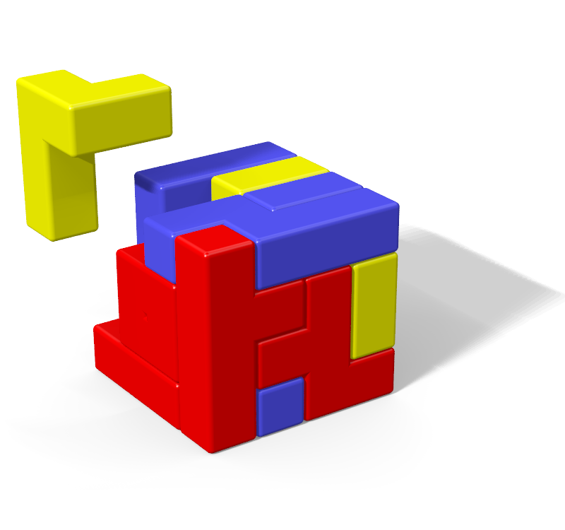
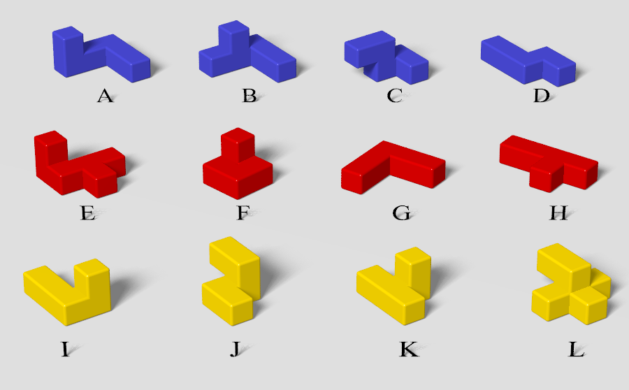
The third set of test cases examines the Tetris Cube puzzle. This puzzle has 12 oddly shaped pieces that must be placed in a 4x4x4 box as shown in Figure 8.
|
|
Test case TC-1 starts like other test cases with DLX, the default S heuristic, and the redundancy filter enabled. Notice that in the TC test group, I supplied the argument L to the -r option. This deserves some explanation. The redundancy filter with no argument given picks a uniquely shaped piece that does the best job of eliminating rotationally redundant solutions by rotationally and/or translationally constraining that piece. If multiple pieces are equally effective in this regard, then it picks a piece among those candidates that have the minimum number of constrained images. I no longer think this is the best rule to use as a tie-breaker. I now believe that instead picking a piece that is large and/or complicated may be a better choice.This makes intuitive sense — it's easier to place the large hard pieces first, and then fill in the smaller more flexible pieces around the big complicated piece, than to place the little easy pieces first and then hope you happen to form a void that the large complicated piece happens to fit nicely into. For example, people who have spent significant time playing with pentomino puzzles know that piece X is difficult to place, and hence it makes a good choice for constraint. I'm not sure how to gauge what makes a piece 'complicated', and so I have not yet tried to modify polycube's selection criteria. In any case, my auto-selection routine, does not always make the best choice for the piece to rotationally and/or translationally constrain to eliminate rotationally redundant solutions. Stephan Westen discovered that piece L in the tetris cube is a much better choice, so in this example I'm passing piece L as the argument to the -r option to force the redundancy filter to constrain that piece to eliminate rotationally redundant solutions. Under this configuration, the solver found all 9839 solutions in about 1 minute 58 seconds. Pieces were placed in the box (and subsequently removed) around 30 million times.
Test case TC-2 enables FILA after DLX places the first piece, and also switches from the S heuristic to my E heuristic at the same time (as described above). Notice that the number of fits increases by about 60% to 49 million indicating the E heuristic does not do as good a job of picking the minimum fit target. The number of no-fit images found by searchFila also increases from 0 to over a billion, and this does not count the vastly larger number of fit checks performed by the e-heuristic itself. But despite these extensive activities and degraded ability to pick the minimum fit target, use of FILA with the E heuristic yields a better than 5-fold increase in solver performance, reducing the total run time by 80.3% down to just 22.2 seconds.
Test case TC-3 swtiches from the E heuristic to the much lighter weight F heuristic when only 3 pieces remain. All the time spent counting neighbor holes at each remaining cell, and then doing fit-counts for those candidate cells with a minimum number of open neighbors just can't pay off when there are so few pieces left. You are better off just placing pieces as fast as you can with the light weight F heuristic. This again increases the number of image fits by 65% to 80 million, and the number of no-fit images to 1.5 billion, but actually reduces the run time by another 10.2% down to 19.9 seconds.
Test case TC-4 enables NOF filtering, which reduced no fit images by 74% from 1.5 billion down to just 393 million. Note that NOF not only reduces the number of fit checks made by searchFila, but also the fit-checks made by the E heuristic. This efficiency in image processing reduced run time by 14.7% to just 17.0 seconds.
Test Case PT: Pentominoes + Tetrominoes in a 13x13 Diamond
Test case PT examines the problem of placing the 12 pentominoes and 5 tetrominoes into a diamond shaped puzzle measuring 13 squares wide and 13 high as shown in Figure 7. Five squares are eliminated from the center to achieve the correct volume.
Test case PT-1 uses DLX, with the S heuristic, and the redundancy filter enabled. All 51,184 unique solutions are discovered in about 10 minutes 46 seconds.
Test case PT-2 enables the volume filter, but instead of only applying the filter once at the beginning, the volume filter is reapplied after every piece placement until fewer than 13 pieces remain to be placed. This technique is particularly effective on this puzzle because the jagged puzzle edges and the central island make it susceptible to partition. This produced a better than 3-fold improvement in solver speed, reducing the total run time by 72% down to just 3 minutes 2 seconds.
Test case PT-3 enabled FILA and the estimate heuristic when 13 pieces remain, reducing the run time by another 62% down to just 1 minute 10 seconds.
Test case PT-4 uses the lighter weight F heuristic for the last 3 piece placements giving an additional small performance improvement of 3.6%, reducing the total run time by another 2 seconds down to 1 minute 8 seconds.
Test case PT-5 enabled NOF. No fit images were reduced by 76% (the largest percent reduction seen over all test cases examined in this document), and run time was reduced by another 10.5%, down to 1 minute 1 second.
Micro FILA Performance Characteristics
Let's focus on just test case P-4 where FILA was used with the F heuristic without NOF enabled to solve the pentominoes 10x6 problem. The informational output from that run includes the following:
# Number of placement attempts when N pieces were left to be placed:
ATTEMPTS[ 1]=        301677
ATTEMPTS[ 2]=       3478035
ATTEMPTS[ 3]=       5722296
ATTEMPTS[ 4]=       3665538
ATTEMPTS[ 5]=       1284992
ATTEMPTS[ 6]=        386776
ATTEMPTS[ 7]=        200366
ATTEMPTS[ 8]=        126819
ATTEMPTS[ 9]=         28279
ATTEMPTS[10]=          3088
ATTEMPTS[11]=           131
ATTEMPTS[12]=             7

# Number of fits when N pieces were left to be placed:
FITS[ 1]=              2339
FITS[ 2]=            302256
FITS[ 3]=            760374
FITS[ 4]=            617667
FITS[ 5]=            272072
FITS[ 6]=             82406
FITS[ 7]=             26950
FITS[ 8]=             17275
FITS[ 9]=              7994
FITS[10]=              1744
FITS[11]=               131
FITS[12]=                 7
This output gives, as a function of the remaining number of pieces $p$, the number of times the solver tried to place a piece in the puzzle (ATTEMPTS), and how many times it actually succeeded in placing a piece in the puzzle (FITS). We can learn a lot from this information through some simple calculations. This program output is transcribed to the second and third columns of Table 2. Subtracting fits from attempts gives the no-fits information in the fourth column. Note that each time a piece is successfully placed in the puzzle when, say, 5 pieces were left, produces a recursive invocation of solveFila with the number of remaining pieces $p$ reduced by 1 to 4. So by dividing the total number of attempts when 4 pieces were left (3,665,538) by the total number of fits when 5 pieces were left (272,072), gives the average number of piece fitting attempt events per cell (or piece) targeted by a single recursive call solveFila when $p = 4$: (3,665,538 / 272,072 = 13.473). Similarly, dividing the total number of fits or no-fits when $p$ pieces are left by the total number of fits when $p+1$ pieces are left, yields the number of times a piece fit or (respectively) didn't fit per target when $p$ pieces were left. This information is tabulated in the last three columns of Table 2 as attempts-per-target, fits-per-target, and no-fits-per-target.
Table 2. Piece placement attempt, fit, and no-fit statistics for test case P-4.
|
Table 3. Piece placement attempt, fit, and no-fit statistics for test case P-5.
|
Table 3 gives the same information as Table 2 but for test case P-5 where NOF was enabled. Compare tables 2 and 3 to verify that NOF doesn't affect fits at all — rather it only reduces the number of images that don't fit in the puzzle that must be processed by each recursive invocation of solveFila. Comparing the last column of Table 2 with the last column of Table 3, shows the level to which NOF filtering reduces the number of no-fit images for each invocation of solveFila. As can be determined from column fits-total, over 93% of solveFila invocations are for $p$ values from 1 to 5. In this range, when NOF is enabled, the total number of images that must be considered is (in the worst case) only about 8. Of these 8, less than 5 are no-fit images. So of the original 63 images that de Bruijn examined at every recursive step of his algorithm, FILA with NOF only has to look at 8, and almost half of these do actually fit. Why so few images?
Many images are eliminated on a cell-by-cell basis due to puzzle bounds considerations: of the $63 \times 60 = 3780$ images that one could try to place at the 60 puzzle cells, only 2056 are bounded by the puzzle walls. The rotational redundancy filter reduces the number of allowed placements of the X piece by 24 (from 32 down to 8). The volume filter eliminates another 125 images (including one of the remaining X images), reducing the total number of images down to $2056-24-125=1907$. Recall that DLX is used to place the X piece in one of 7 starting locations in the lower left quadrant. Each such placement eliminates a large number of images (primarily from the left side of the puzzle) from the DLX matrix. For example, the last such placement (when the X piece is placed very close to the center of the puzzle) leaves the matrix with only 1101 images. These 1101 images are then used to populate the matrix of image list sets $A$ used by FILA. POF filtering would nominally keep the total number of images in each image list set to 63, but all of the other reductions to this point makes these lists on average much smaller. For the case where only 1101 DLX images remain after placing the X piece for the last time, POF reduces the average number of images per image list set over the remaining 55 holes to just $1101 / 55 \approx 20.0$. This average of 20 is not typical since, for example, the image list sets for cells near the X piece and near the right border wall will have fewer images. Likewise cells just to the right of the X will have significantly more than the average 20. When work is most intense (when 4 pieces are left) about an additional 8/12 (67%) of these images are discounted simply because 8 pieces are unavailable (and so their images are never attempted). Finally, NOF filtering reduces the no-fit images in the image list sets by (on average) another 64.3% (as seen from test case P-5 in Table 1) to produce the overall sizes seen here in Table 2.
After all this reduction, remember that each of the few remaining no-fit images that still have to be considered, are ruled out by a single machine instruction that performs a binary-and of the puzzle occupancy state with the layout-bit-mask of the image (line 11 of solveFila). I am skeptical, therefore, that more specialized NOF image lists based on the occupancy states of additional neighbors near the target cell, could possibly reduce no-fit images in sufficient number that the resulting reduction in image fit-check processing time could outweigh the increased processing time needed to calculate the more detailed ILSI. And this does not even consider the increased initialization times to generate the larger number of image list sets in $A$ (which grows by a factor of 2 for each additional neighbor considered).
Tables 4 and 5 provide the same piece-by-piece and per-target statistics for test cases TC-3 and TC-4 of the Tetris Cube. I won't bore you with as much detail here, but I wanted to impress upon you the usefulness of NOF when used in combination with the E heuristic and in higher dimensional puzzles (3D instead of 2D). Compare, for example, the number of no-fits-per-target when 4 pieces remain from tables 4 and 5: by enabling NOF, the number of no-fit images is reduced from 27.7 all the way down to 3.2 — a reduction factor of 8.6. There are two reasons for this this large reduction. First, the E heuristic is not an ordered heuristic, so no POF filtering is possible. Where for the pentominoes puzzle, there are only 63 images to choose from to populate the image list sets; the lack of POF filtering, and the increased rotational freedom results in 1416 Tetris Cube piece images that could possibly populate each image list set at a cell. Again, puzzle boundary considerations, the rotational redundancy filter, and the placement of the first piece by DLX, will drastically reduce the numbers of available images by the time FILA is actually activated, but we are still left with much larger image list sets. Because the E heuristic always targets a cell with a maximum number of occupied (or non-existent) neighbors, it naturally targets cells that produce ILSI with many bits set, for which NOF filtering is most effective. Because no POF filtering is possible, all filtering is due to NOF — which makes NOF just all that more useful for heuristics that don't follow a fixed targeting order.
Table 4. Piece placement attempt, fit, and no-fit statistics for test case TC-3.
|
Table 5. Piece placement attempt, fit, and no-fit statistics for test case TC-4.
|
Performance Comparison of polycube 2.0 and polycube 1.2.1
Although NOF does seem to consistently provide a significant performance improvement, there were other software implementation changes that provided even greater performance benefits. Most significantly, the old EMCH algorithm counted open neighbors one neighbor at a time. FILA's new E heuristic uses either a silicon based bit population count instruction (if available) or table-based lookups to count the number of neighbor holes at each cell which is far faster. Similarly, my old variation of the de Bruijn algorithm iterated over the heads of the DLX matrix to find unoccupied cells. It did remember where it last left off (so it wasn't starting from the beginning with each request), but FILA's new F heuristic more efficiently iterates over the occupancy bit field looking for zeroes. It can use silicon based instructions (if available) or table lookups to do this efficiently. These and other small optimizations together with NOF have improved the solve times for some puzzles by almost a factor of two. For example, the best solve time I can produce with polycube version 1.2.1 for the Tetris Cube is 31.6 seconds. Version 2.0 solves the same puzzle on the same machine in just 17.0 seconds (as noted above), a reduction in run time of 46%. 2D puzzle performance (for which the E heuristic is not typically most useful), has improved by a lesser, but still significant amount. For example the best solve times for the pentominoes 10x6 puzzle have improved on my machine from about 0.212 seconds down to 0.156 seconds — a 26% improvement.
Future Work
FILA Ordering Heuristics that Target Pieces
There's nothing in the FILA-heuristic interface that precludes a heuristic from targeting a piece (rather than a cell) and returning an image list set that lists only images for a single target piece. Unfortunately, if a heuristic is targeting pieces, then it cannot be a fixed-order heuristic, which means you can't use POF to gradually reduce the size of the image list sets that target pieces as the puzzle is filled in. And NOF filtering alone would be almost completely useless for reducing the size of image list sets that target pieces. So I don't immediately see a way to, for example, extend the estimate heuristic to efficiently identify pieces that have few fits and/or identify a precalculated image list targeting such a piece that is well filtered to the current puzzle state. Still, there may be times that targeting pieces could be useful, even if it requires much work to identify the target (e.g., fit-counting across all images of a piece), and even if the returned image list set is not well filtered (e.g., just return all images of the piece with no filtering at all). Such an approach might still perform favorably compared to DLX within some limited range of puzzle sizes.
Also, for the special case where the puzzle solve is just getting started ($p = P$), every image in all image list sets are guaranteed to fit. So the S and E heuristics could easily be modified to notice that $p = P$ and instead of counting fits or neighbor holes, just look at the list sizes. Image list sets that target pieces could be included specifically for this situation, so that FILA could target, for example, a piece that's been highly constrained to eliminate rotationally redundant solutions. This would enable FILA to fully emulate de Bruijn and Fletcher for the 10x6 pentomino problem by identifying that the X piece should be placed first. It is not clear to me, however, that there would be any advantage to this approach over my current approach of always using DLX to place the first piece of a puzzle (other than the elimination of DLX itself — which is obviously no small simplification.) In fact, it is my expectation that such an approach would be inferior to the current approach of using the combination of algorithms: In the 10x6 pentomino problem, placing the X piece smack in the middle of the puzzle causes DLX to eliminate many images. Using this reduced image set as a feed for the initialization of the fixed image list sets used by the FILA F heuristic is highly advantageous and this is not a behavior that a pure FILA approach to the problem can readily replicate.
For now, I leave the subject of defining FILA ordering heuristics that can target pieces as a problem for future investigation.
Code Generation
I have not definitively answered the question of whether FILA is faster than Fletcher's algorithm for the 10x6 pentomino problem. I have not even taken the time to translate Fletcher's original program to a modern programming language. But even if I did, a comparison between that program and polycube wouldn't really be a fair comparison of Fletcher's algorithm and FILA: Fletcher's program is hard coded to solve the 10x6 pentomino puzzle which has several advantages:
- much indirection and array indexing can be eliminated;
- for-loops can be unrolled;
- simplifications are made possible due to all pieces being the same size; and
- simplifications are made possible due to all pieces having a different shape.
Because polycube is a general puzzle solver, it is necessarily more cumbersome. As a result, Fletcher's program is not only simpler, but also smaller, which allows for better CPU caching. So if someone were to compare a direct translation of Fletcher's published software to polycube 2.0 and reported Fletcher's software faster I would be neither surprised, nor deterred.
To make a more-fair comparison, I could add some generalization of Fletcher's algorithm to polycube. This would not only require finding an algorithm to efficiently assign images to a search tree, it also would require (I think) a new data model since Fletcher's algorithm requires checking the occupancy of cells just outside the puzzle boundary — something polycube doesn't currently allow. I guess I'm not interested in such an endeavor — especially since the results would not necessarily be definitive.
Alternatively, one could write a code generator that takes a puzzle as input and outputs a FILA solver program that's hard-coded and highly optimized to the particulars of the input puzzle. Such a program generated for the 10x6 pentomino problem could, I think, then be fairly compared to Fletcher's original hard-coded program for the same puzzle (with only those minimal modifications needed to translate it to a modern programming language). I suspect such an optimized FILA solver could be made to run far faster than Fletcher's original program. The more I think about this, the less hard it seems like it would be to do. Maybe I'll try it some time — not to prove FILA faster than Fletcher at pentominoes 10x6 (something I already believe to be true), but rather to be able to solve harder puzzles more efficiently.
Applications to Other Geometries
polycube 2.0 is restricted to puzzles whose cells fall on the integer lattice points of a two or three dimensional Cartesian coordinate system, but there is nothing about the FILA algorithm or POF or NOF filtering that is limited in this way. (The calculation of the ILSI given here does talk about the nearest neighbors in the 6 ordinal directions, but in general a neighbor can be in any direction, and the mapping of those neighbors to ILSI bits is arbitrary.) Other puzzle geometries, like polyiamonds, polyhexes, and polysticks could also be solved with a FILA software application that was suitably abstracted to service those geometries.
Software Download
This software is protected by the GNU General Public License (GPL) Version 3. See the README.txt file included in the zip file download for more information.
- LICENSE.txt (GNU General Public License Version 3)
- README.txt (Copyright, build and run instructions)
- RELEASE_NOTES.txt (Summary of changes for each release)
- polycube.exe (polycube solver executable for Windows 64 bit processors)
- Several sample puzzle definition files including all puzzles used in my web docs, and others.
- polycube 2.0 C++ source code.
- A small subset of boost c++ library source (only those packages used by polycube).
- double precision SIMD oriented Fast Mersenne Twister (dSFMT) source code (for random number generation).
Contents: same as for Windows, but no executable is provided, and all text files are carriage return stripped.
The source is about 16,000 lines of C++ code, with dependencies on two other libraries (boost and the Mersene Twister random number generator) which are also included in the download. The executable file polycube.exe is a Windows console application (sorry, no GUIs folks). For maximum platform compatibility, the provided executable has NOT been compiled to use g++ builtin bit-field operations __builtin_popcount() or __builtin_ctz(). If you make the effort to compile for your own hardware (see README.txt), you should see a moderate performance improvement to FILA. I've seen 8% to 15% depending on the puzzle and the heuristics used.
Conclusions
FILA is a fast flexible recursive backtracking algorithm that uses precalculated (fixed) lists of images that are pre-filtered to exclude images incompatible with the cells location, incompatible with cells that must have been previously filled by a heuristic (POF), or incompatible with occupancy states of the nearest neighbors of the targeted cell (NOF).
Fletcher and de Bruijn used a fixed list of 63 pentomino images that were considered for placement at each targeted cell in the 10x6 pentomino problem, but many of these images collide with puzzle walls. By using a separate list of images at each cell, images that lie partially outside the puzzle bounds can be eliminated. For this puzzle, this reduces the number of images in each list by on average 45.6%.
Fletcher and de Bruijn recognized that by filling a puzzle from left to right using a strict cell selection order, the number of images that had to be considered at each cell was greatly reduced (80%). POF filtering generalizes this technique to any heuristic that targets cells in a predetermined order, eliminating all images that conflict with cells that must have been filled prior to the targeted cell.
Instead of considering all images in a set one-at-a-time, Fletcher walked the cells near a fill target to eliminate images in groups. Instead of walking the whole tree (sections of which often correspond to regions outside the puzzle boundary, or to pieces that are not even available), NOF focuses on just the most important nearest neighbor cells, aggregating their occupancy states into a small index number used to select a set of images built specifically for that compound neighbor occupancy state. This approach eliminates on average an additional two-thirds to three-fourths of the images that don't fit the puzzle.
The combination of these three strategies eliminates the vast majority of images that don't fit the target. For example, for the solver configuration that produced fastest solve times for the Tetris Cube, the F heuristic (Fletcher's heuristic) was used when 3 pieces were left to be placed. The average number of images that had to be considered by a single recursive invocation of the algorithm at that stage was just 11.3; and the number of these images that didn't fit was just 9.2. This is as compared to the 1,416 unique tetris cube piece images that would populate these lists if no filtering was used at all. NOF filtering is particularly useful for unordered heuristics (where POF filtering is not possible). For the same tetris cube solver configuration, the E heuristic was used when 4 pieces were left to be placed. The average number of images that had to be considered at this stage was only 4.3 with only 3.2 of those images not fitting. So through these simple techniques the lion's whale's share of images that don't fit are eliminated from the algorithm at the cost of checking the occupancy states of at most a few cells. (This is as compared to DLX's higher-cost approach of dynamically maintaining perfect image lists with every piece placement or removal.) The net effect is faster solve times. The NOF feature alone improved solve times 6% to 17% for the puzzles examined here (though I have seen as high as 27% in other puzzles).
References
- D. Knuth. Dancing Links. In J. Davies, B. Roscoe, and J. Woodcock, editors, Millennial Perspectives in Computer Science, proceedings of the 1999 Oxford-Microsoft Symposium in honour of Professor Sir Antony Hoare, Cornerstones of Computing, page 432. Palgrave Macmillan, 2000.
- J.G. Fletcher. A program to solve the pentomino problem by the recursive use of macros. Communications of the ACM, 8(10):621–623, 1965.
- N.G. de Bruijn. Programmeren van de pentomino puzzle. Euclides 47 (1971/72), 90-104.
- M. Busche. Solving Polyomino and Polycube Puzzles; Algorithms, Software, and Solutions. Matt's Maniacal Musings, 2011.
I downloaded and compiled your latest version of polycube and compiled it using your README File. I will update my website to reflect your latest execution times on my computer. Thanks for sharing your program and advanced research.
I ran polycube2.0.1 as follows on my new (old) desktop computer:
HP-8300 Windows 10 Home i5-3470 @ 3.2GHz as follows:
polycube -i -q -r -V -of=11 -f11 -n .\def\pentominoes_10x6.txt
Using FILA, polycube2.0.1 found the 2339 solutions to the 10×6 puzzle in .22 secs. My fastest solver, fletcher4ns.c, also runs in .22 secs and bruijn.c, which is just a translation of N.G de Bruijn’s Algol60 code, solves the 10×6 puzzle in .33 secs. FILA very well may be an even more efficient algorithm than the standards established about 50 years ago by John G. Fletcher and N.G. de Bruijn. Thanks for sharing your source code and ideas.
Hello Matt. I have been using your software since May of 2014 when it was 1.1.3. Last summer I managed to catch your 2.0 version (then your site vanished for a bit which was disturbing) and was once again able to compile it easily. I was having a harder time with the 1.2 version over time on Debian so that was great. These new versions seem blazingly fast and I’ve even compiled it for my raspberry pis (zeroW, 3 and 3a+).
While I don’t really understand the math (or much of your explanations in general) I was able to use the solver to create a specialized set of packing puzzles that take 10 pieces and create 2 3x3x3 cubes with only one solution. Thanks to the solver (and a frightening set of bash scripts I banged together over the years) I have 365 unique puzzle pair sets.
So thank you. If you are interested I’d be happy to pass along the compiled raspberry binaries built with a gcc 8.1 cross compiler. The 2.0.2 version is only 884k unstripped. The same binary runs on all three of those raspberries. Your work is much appreciated.
Well thankyou for your thankyou! I’ve had many thousands of downloads from real people (I filter out robots in my stats as best I can), but very few take the time to even leave comment. I appreciate it.
Out of curiosity, was your objective to produce a small and difficult puzzle with only one solution? Sometimes puzzles with only one solution have so many constraints that the solution will reveal itself easily. I too have spent time trying to construct puzzles that are very difficult to solve. I measure difficulty by looking at the ratio of the number of solutions found to the number of times pieces are placed in the puzzle by the solver. The most difficult puzzle I’ve constructed is based on the 29 pentacubes: it took my solver several days to find the first solution. (I was about to give up thinking it unsolvable.)
I know the older versions of my code don’t compile well with the newer compilers. I should probably clean them up, but I’m not sure why anyone would want to compile the older versions of the software so I haven’t messed with it.
I appreciate the offer of the raspberry pi binary, but I’m so paranoid about trojans and viruses from stuff I download from the internet, I can’t in good conscience post a binary from a third-party on my website. (Frankly, I think people are nuts for running my binaries instead of compiling the source for themselves — maybe the fact that I’m open about who I am and where I live gives them some assurance I’m not up to something nefarious.)
As far as my site going down, here’s the story: I got tired of Comcast raising my monthly bill every couple of months, and so I finally dumped them. I switched to Century Link. They guaranteed me no rate hikes for life. They’ve been fine, but they seem to reboot their routers every couple of weeks, and they apparently don’t persist DHCP address assignments (so that no attempt can be made to assign the same addresses to DHCP clients after the reboot). So every reboot causes a DHCP IP address reset, which takes down my site until I notice the problem and update the DNS mapping. This issue is exacerbated by the fact that their in-home router software is not very good — it can’t correctly forward packets from computers behind the firewall to a local server using it’s public-facing DNS alias. (That is, I can’t reach my own server using the address http://www.mattbusche.org — I have to hard-code an entry for http://www.mattbusche.org in my /etc/hosts files so it uses the local IP address.) And this effectively hides the fact that the site was down. Sadly, their latest DSL modem technology is not yet available from a third-party, so I’m stuck with their quirky box for now.
Now I could have avoided all this by paying Century Link an extra 10 bucks a month to get a fixed IP address, but I’m poor (or perhaps I’m just cheap). Instead, I wrote a script (a rewrite of something I found on the internet) that once-a-minute looks for a local IP address change, and when detected will dynamically update the DNS entry for http://www.mattbusche.org. This new script has already fixed things for me a couple of times. It seems to be working beautifully.
I also added something to my bash .profile to verify things are good and print out an obnoxious banner when things are awry. So even if my script should fail, I’ll notice the problem the next time I login.
Anyway, the address changes should now be corrected within 2-3 minutes (depending on Century Link router boot time), but you might see an outage for longer (maybe half an hour-ish) due to DNS caching. Usually this happens in the wee-hours, so if you’re in the western hemisphere, it probably won’t affect you in any case.
I should add some advertising to my site and maybe I could make enough money to pay for the fixed IP address. 🙂
The whole Battle with the Cable Provider made me laugh. I worked as a coax splicer, field engineer, lineman for about 20 years and have worked as a contractor with all the major names and quite a number of minor ones. The reason I finally left it all is because of how ridiculous they have become. When I worked in house for a smaller one in PA I went from doing RF design on the fly to changing modems. Yeah, no love lost there. Your system around them is delightfully demented. I can get behind that sort of thing!
So, the puzzles. I was in a new country with my wife finishing school at home with our new baby. I read an old book (some Project Gutenberg scan) about puzzles and it led me to Mikusinski’s cube and probably Stewart Coffin’s book. (ah, this stuff here https://johnrausch.com/PuzzlingWorld/chap03.htm) Since I had no wood shop and was playing around with Tomoko Fuse’s modular origami, I had discovered a way to make polycubes that were stable enough to play with. Idle hands and all. With all that I had the basics for making puzzles but no way to figure out if they had solutions or how to find them etc. After a bunch of trial and error quests I found BurrTools. Since the Rhombic Tetrahedra looked exactly like the surfaces of the paper cubes I made out of paper modules. I could model them in a way that was pretty sane. But, I couldn’t use it’s solver from the command line. So once I got past just making a few puzzles I ended up on a quest to make something unique. Then I found out just how many permutations can dance on the head of a pin.
Anyhow…I needed something to run from a script and your program was pretty much perfect for what I needed.
What I ended up doing was seeing what shapes I liked. I decided on something that would always fit into a 2×3 footprint and extend at least one cube up, never touching edges in a way that left a socket. Nor could they have Rotational symmetry so the surface patterns couldn’t be messed up while solving. After some trial and error I boiled my polycube parade down to 2 made of 7 cubes, 7 made of 6 cubes and 9 made of 5 cubes. I tossed the 7 cube ones since, well, 27, and settled on the 6-6-5-5-5 pattern. Pretty much then lots making giant lists of permutation groups, whittling them down, etc etc. Once I had all the 3x3x3 cubes that could be made I sorted out the groups of 10 pieces that could both make cubes, I had to sort out the ones that only had one solution and only one way to create 2 cubes.
So, you can image, I made heavy use of your program since it was easy to parse the output. Granted, I could have saved myself about 3 man lifetime hours by using an actual language but bash scripts are that dirty nasty thing that you just can’t put down. But, tons of time and after a lot of trying I got my puzzle pairs. Crazily I had 364 of them. So, Year of Puzzles was born.
That was a long way to address your question of complexity. How about I just give you an example of what your program helped to wrought. 😛
Hmm, no way to attach a file. Okay, I’ll just put it in the next comment if you want to give it a go.
Long, story longer, in the end I think I sort of sculpted with math. Just because I don’t understand all the math doesn’t mean I can’t make something beautiful with it. 🙂
So the next comment is my testing script. You can also see what pieces I ended up using for my set.
There are many puzzles where all pieces have the same shape. For example, using 25 copies of the Y pentomino to fill a 5x5x5 box. Relative to other puzzles having many piece shapes, puzzles with only one piece shape have far fewer fit choices for any given fill target. I have discovered that NOF filtering does not help with theses types of puzzles, and can actually slow things down significantly. When I have time, I may update this document to include a test case for such a puzzle to highlight situations where NOF filtering makes things worse.