I've implemented a set of backtrack algorithms to find solutions to various polyomino and polycube puzzles (2-D and 3-D puzzles where you have to fit pieces composed of little squares or cubes into a confined space). Examples of such puzzles include the Tetris Cube, the Bedlam Cube, the Soma Cube, and Pentominoes. My approach to the problem is perhaps unusual in that I've implemented many different algorithmic techniques simultaneously into a single puzzle solving software application. I've found that the best algorithm to use for a problem can depend on the size, and dimensionality of the puzzle. To take advantage of this, when the number of remaining pieces reaches configurable transition thresholds my software can turn off one algorithm and turn on another. Three different algorithms are implemented: de Bruijn's algorithm, Knuth's DLX, and my own algorithm which I call most-constrained-hole (MCH). DLX is most commonly used with an ordering heuristic that picks the hole or piece with fewest fit choices; but other simple ordering heuristics are shown to improve performance for some puzzles.
In addition to these three core algorithms, a set of constraints are woven into the algorithms giving great performance benefits. These include constraints on the volumes of isolated subspaces, parity (or coloring) constraints, fit constraints, and constraints to take advantage of rotational symmetries.
In this (rather long) blog entry I present the algorithms and techniques I've implemented and share my insights into where each works well, and where they don't. You can also download my software source, an executable version of the solver, and the solutions to various well known puzzles.
Contents
Motivation
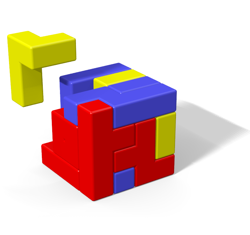
My original impetus for writing this software was an annoyingly difficult little puzzle called the Tetris Cube. The Tetris Cube consists of the twelve oddly-shaped plastic pieces shown in Figure 1 which you have to try to fit into a cube-shaped box. Each piece has a shape you could make yourself by sticking together little cubes of fixed size. You would need 64 cubes to make them all and accordingly, the puzzle box measures 4x4x4 — just big enough to hold them all. (This is an example of a polycube puzzle: a 3-D puzzle where all the pieces are formed from little cubes. We'll also be looking at polyomino puzzles: 2-D puzzles where all the pieces are formed from little squares.)
The appeal of the Tetris Cube to me is three-fold. First, it's intriguing (and surprising to most folks) that a puzzle with only twelve pieces could be so wicked hard. I had spent much time in my youth looking for solutions to the far simpler (but still quite challenging) two-dimensional Pentominoes puzzle, so when I first saw the Tetris Cube in a gaming store about three years ago, I knew that with the introduction of the third dimension that the Tetris Cube was an abomination straight from Hell. I had to buy it. Since then I've spent many an hour trying to solve it, but I've never found even one of its nearly 10,000 solutions manually.
Second, I enjoy the challenge of visualizing ways of fitting the remaining pieces into the spaces I have left, and enjoy the logic you can apply to identify doomed partial assemblies.
Third, I think working any such puzzle provides a certain amount of tactile pleasure. I should really buy the wooden version of this thing.
But alas, I think that short of having an Einstein-like parietal lobe mutation, you will need both persistence and a fair amount of luck to find even one solution. If I ever found a solution, I think I'd feel not so much proud as lucky; or maybe just embarrassed that I wasted all that time looking for the solution. In this sense, I think perhaps the puzzle is flawed. But for those of you up for a serious challenge, you should really go buy the cursed thing! But do yourself a favor and make a sketch of the initial solution and keep it in the box so you can put it away as needed.
Having some modest programming skill, I decided to kick the proverbial butt of this vexing puzzle back into the fiery chasm from whence it came. My initial program, written in January 2010, made use of only my own algorithmic ideas. But during my debugging, I came across Scott Kurowski's web page describing the software he wrote to solve this very same puzzle. I really enjoyed the page and it motivated me to share my own puzzle solving algorithm and also to read up on the techniques others have devised for solving these types of puzzles. In my zeal to make the software run as fast as possible, over the next couple of weeks I incorporated several of these techniques as well as a few more of my own ideas. Then I stumbled upon Donald Knuth's Dancing Links (DLX) algorithm which I thought simply beautiful. But DLX caused me two problems: first it used a radically different data model and would not be at all easy to add to my existing software; second it was so elegant, I questioned whether there was any real value in the continued pursuit of this pet project.
Still I wasn't sure how DLX would compare to and possibly work together with the other approaches I had implemented. The following November, curiosity finally got the better of me and I began to lie awake at night thinking about how to to integrate DLX into my polycube solver software application.
Backtrack Algorithms
The popular algorithms used to solve these types of problems are all recursive backtracking algorithms. With one algorithm that falls in this category you sequentially consider all the ways of placing the first piece; for each successful placement of that piece, you examine all the ways of placing the second piece. You continue placing pieces in this way until you find yourself in a situation where the next piece simply won't fit in the box, at which point you back up one step (backtrack) and try the next possible placement of the previously placed piece. Following this algorithm to its completion will examine all possible permutations of piece placements including those placements that happen to be solutions to the puzzle. This approach typically performs horribly. Another similar approach is to instead consider all the ways you can fill a single target open space (hole) in the puzzle; for each possible piece placement that fills the hole, pick another hole and consider all the ways to fill it; etc. This approach can also behave quite badly if you choose your holes willy-nilly, but if you make good choices about which hole to fill at each step, it performs much better. But in general you can mix these two basic approaches so that at each step of your algorithm you can either consider all ways to fill a particular hole, or consider all ways to place a particular piece. Donald Knuth gives a nice abstraction of this general approach that he dubbed Algorithm X.
Puzzle Complexity
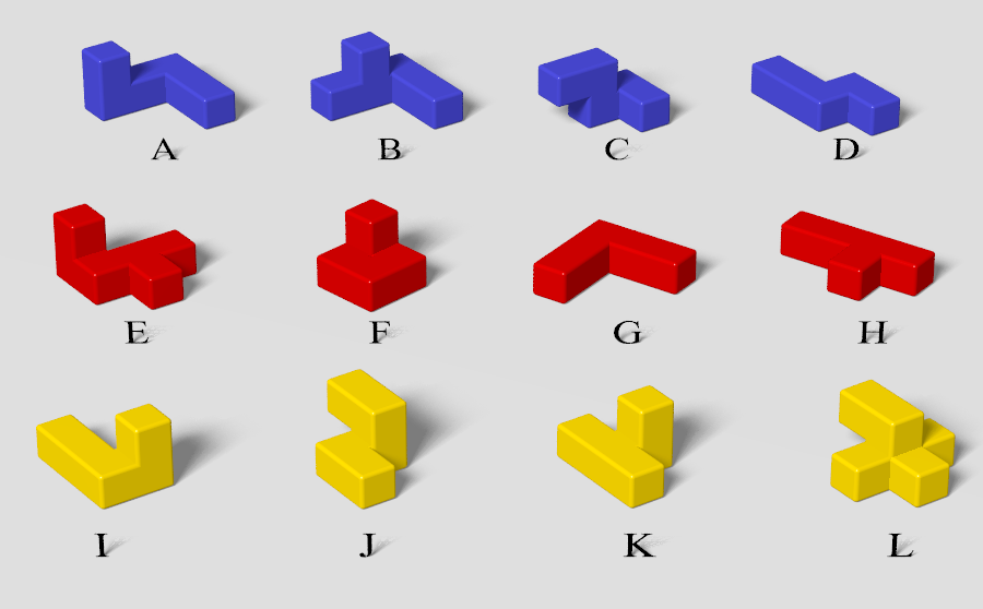
To appreciate the true complexity of these types of problems it is perhaps useful to examine the Tetris Cube more closely. First note that most of the pieces have 24 different ways you can orient (rotate) them. (To see where the number 24 comes from, hold a piece in your hand and see that you have 6 different choices for which side faces up. After picking a side to face up, you still have 4 more choices for how to spin the piece about the vertical axis while leaving the same side up.) Two of the pieces, however, have symmetries that reduce their number of uniquely shaped orientations to just 12. For each orientation of a piece, there can be many ways to translate the piece in that orientation within the confines of the box. I call a particular translation of a particular orientation of a particular piece an image.
If we stick with the algorithmic approach of recursively filling empty holes to look for solutions, then we'll start by picking just one of the 64 holes in the puzzle cube (call the hole Z1); and then one-by-one try to fit each of the pieces in that hole. For each piece, all unique orientations are examined; and for each orientation, an attempt is made to place each of the piece's constituent cubes in Z1. The size of a piece multiplied by its number of unique orientations I loosely call the complexity of a piece, which gives the total number of images of a piece that can possibly fill a hole. If, for example, a piece has 6 cubes and has 24 unique orientations, then 144 different images of that piece could be used to fill any particular hole. The complexity of the twelve Tetris Cube pieces are shown in Table 1. Each time a piece is successfully fitted into Z1, our processing of Z1 is temporarily interrupted while the whole algorithm is recursively repeated with the remaining pieces on some new target hole, Z2. And so on, and so on. Each time we successfully place the last piece, we've found a solution.
| Piece Name | Size | Unique Orientations | Complexity |
|---|---|---|---|
| A | 6 | 24 | 144 |
| B | 6 | 24 | 144 |
| C | 5 | 24 | 120 |
| D | 5 | 24 | 120 |
| E | 6 | 24 | 144 |
| F | 5 | 24 | 120 |
| G | 5 | 12 | 60 |
| H | 5 | 24 | 120 |
| I | 5 | 24 | 120 |
| J | 5 | 12 | 60 |
| K | 5 | 24 | 120 |
| L | 6 | 24 | 144 |
The number of steps in such an algorithm cannot be determined without actually running it since the number of successful fits at each step is impossible to predict and varies wildly with which hole you choose to fill. It is useful however (or at least mildly entertaining) to consider how many steps you'd have if you didn't backup when a piece didn't fit, but instead let pieces hang outside the box, or even let two pieces happily occupy the same space (perhaps slipping one piece into Buckaroo Banzai's eighth dimension) and blindly forging ahead until all twelve pieces were positioned. In this case, the total number of ways to place pieces is easily written down. There are 12 × 11 × 10 . . . × 1 = 12! possible orderings of the pieces. And for each such ordering, each piece can be placed a number of times given by its complexity. So the total number of distinct permutations of pieces that differ either in the order the pieces are placed, or in the translation or orientation of those pieces is:
That's 2.2 decillion. The total number of algorithm steps would be a more than double that (since each piece placed also has to be removed). But this is just silliness: any backtracking algorithm worth its salt (and none of them are very salty) will reduce the number of steps to well below a quadrillion, and a good one can get the number of steps down to the tens of millions. I now examine some specific algorithms and explain how they work.
De Bruijn's Algorithm
The first algorithm examined was first formulated independently by John G Fletcher and N.G. de Bruijn. I first stumbled upon the algorithm when reading Scott Kurowski's source code for solving the Tetris Cube. To read Fletcher's work you'll either need to find a library with old copies of the Communications of the ACM or drop $200.00 for online access. (I've yet to do either.) De Bruijn's work can be viewed online for free, but you'll need to learn Dutch to read it. (It's on my to-do list.) Despite my ignorance of the two original publications on the algorithm, I'll take a shot at explaining it here. With no intended sleight to Fletcher, from here on, I simply refer to the algorithm as de Bruijn's algorithm. (I feel slightly less foolish calling it de Bruijn's algorithm since I have at least examined and understood the diagrams in his paper.)
De Bruijn's algorithm takes the tack of picking holes to fill. Now I previously said that when filling a hole, that for each orientation of each piece, an attempt must be made to place each of the piece's constituent cubes in that hole; but with de Bruijn's technique, only one of the cubes must be attempted. This saves a lot of piece fitting attempts. To understand how this works, first assume the puzzle is partially filled with pieces. De Bruijn's algorithm requires you pick a particular hole to fill next. A simple set of nested for loops will find the correct hole. The code could look like this:
        GridPoint* Puzzle::getNextBruijnHole()
        {
            for(int z = 0; z < zDim; ++z)
                for(int y = 0; y < yDim; ++y)
                    for(int x = 0; x < xDim; ++x)
                        if(grid[x][y][z]->occupied == false)
                            return grid[x][y][z];
            return NULL;
        }
This search order is also shown visually on the left hand side of Figure 2.
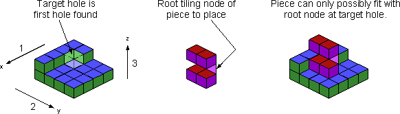
Because of the search order there can be no holes in the puzzle with a lesser z value than the target hole. Similarly, there can be no holes with the same z value as the target hole having a lesser y value. And finally, there can be no hole with the same y and z values as the target hole having a lesser x value.
Now consider a particular orientation of an arbitrary piece like the one shown in the center of Figure 2. Because there can be no holes with a lesser z value than the target hole, it would be pointless to attempt to place either of its two top cubes in the hole. That would only force the lower cubes of the piece into necessarily occupied GridPoints of the puzzle. So only those cubes at the bottom of the piece could possibly fit in the target hole. But of those three bottom cubes, the one with the greater y value (in the foreground of the graphic) can't possibly fit in the hole because it would force the other two bottom tier pieces into occupied puzzle GridPoints at the same height as the hole but with lesser y value. Applying the same argument along the x axis leads to the conclusion that for any orientation of a puzzle piece, only the single cube with minimum coordinate values in z, y, x priority order (which I call the root tiling node of the piece) can possibly fit the hole. This cube is highlighted pink in Figure 2.
So with de Bruijn's algorithm, a piece with 6 cubes and 24 orientations would only require 24 fit attempts instead of 144 at a given target hole. This allows the algorithm to fly through piece permutations in a hurry.
De Bruijn's paper focused on the 10x6 pentomino puzzle, perhaps the most famous of all polyomino and polycube puzzles. The puzzle pieces in this problem consist of all the ways you can possibly stick 5 squares together to form rotationally unique shapes. There are 12 such pieces in all and each is given a standard single character name. Figure 3 shows the twelve pieces with their names as well as one of the 2339 ways you can fit these pieces into a 10x6 box. To be accurate, de Bruijn only used the algorithmic steps described above to place the last 11 pieces in this puzzle. He forced the X piece to be placed first in each of seven possible positions in the lower left quadrant of the box. This was done to eliminate rotationally redundant solutions from the search, and significantly sped up processing. But where possible I'd like to avoid optimization techniques that require processing by University professors. So when I speak of the de Bruijn algorithm, I do not include this special case processing. This restriction significantly weakens the algorithm. (I found it to take ten times longer to find all solutions to the 10x6 pentomino puzzle without this trick.) As I explain later, I've implemented an image filter that can constrain a piece to eliminate rotationally redundant solutions from the search. Applying this filter to the 10x6 pentomino puzzle algorithmically reproduces de Bruijn's constraint on the X piece.
In Figure 4, I've captured an excerpt of de Bruijn's algorithm working on the 10x6 pentomino puzzle at a point where it's behaving particularly badly. It reveals an interesting weakness of the algorithm: it can be slow to recognize a position in the puzzle that's clearly impossible to fill. The algorithm doesn't recognize this problem until it selects the troublesome hole as a fill target, but even then it won't back up all the way to the point where the hole is freed from its confinement: it only backs up one step. So depending on how far away the isolated hole is in the hole selection sequence at the time the hole appeared, it may get stuck trying to fill the hole many many times. Because pentominoes pieces are all fairly small, and because the algorithm uses a strict packing order from bottom to top and from left to right, such troublesome holes can never be that far away from the current fill target and are thus usually discovered fairly quickly. The example I've given may be among the most troublesome to the algorithm, but things can get worse if you are working with larger pieces, or if you are working in 3 dimensions instead of 2. In either case, unfillable holes can appear further down the hole selection sequence and the algorithm can stumble over them many more times before the piece that created the problem is finally removed.
The next algorithm examined does not suffer from this weakness.
Dancing Links (DLX) Algorithm
Dancing Links (DLX) is Donald Knuth's algorithm for solving these types of puzzles. The DLX data model provides a view of each remaining hole and each remaining piece and can pick either a hole to fill or a piece to place depending on which (among them all) is deemed most advantageous.
DLX Description
Knuth's own paper on DLX is quite easy to understand, but I'll attempt to summarize the algorithm here. Create a matrix that has one column for each hole in the puzzle and one column for each puzzle piece. So for the case of the Tetris Cube the matrix will have 64 hole columns + 12 piece columns = 76 columns in all. We can label the columns for the holes 1 through 64, and the columns for the pieces A through L. The matrix has one row for each unique image. (Only images that fit wholly inside the puzzle box are included.) If you look at one row that represents, say, a particular image of piece B, it will have a 1 in column B and a 1 in each of the columns corresponding to the holes it fills. All other columns for that row will have a 0. (Those are the only numbers that ever appear in the matrix: ones and zeros.) Now, if you select a subset of rows that correspond to piece placements that actually solve the puzzle, you'll notice something interesting: the twelve selected rows together will have a single 1 in every column. And so the problem of solving the puzzle is abstracted to the problem of finding a set of rows that cover (with a 1) all the columns in the matrix. This is the exact cover problem: finding a set of rows that together have exactly one 1 in every column. With Knuth's abstraction there is no distinction between filling a particular hole, or placing a particular piece; and that is truly beautiful.
In each iteration of the algorithm, DLX first picks a column to process. This decision is rather important and I discuss it at length below. Once a column is selected, DLX will in turn place each image having a 1 in that column. For each such placement, DLX reduces the matrix removing every column covered by the image just placed, and removing every row for every image that conflicts with the image just placed. In other words, after this matrix reduction, the only rows that remain are for those images that still fit in the puzzle, and the only columns that remain are for those holes that are still open and for those pieces that have yet to be placed. Knuth uses some nifty linked list constructions to perform this manipulation, which you can read about in his paper if interested.
DLX maintains the total number of ones in each column as state information. If the number of ones remaining in any column hits zero, then the puzzle is unsolvable with the current piece configuration and so the algorithm backtracks. The situation in Figure 3 that gave the de Bruijn algorithm so much trouble gives DLX no trouble at all: it immediately recognizes that the matrix column corresponding to the hole that can't be filled has no rows with a one and backtracks, removing the piece that isolated the hole immediately after it was placed.
Some benefits of DLX are:
- the elimination of all processing associated with "checking" to see if a particular image fits (which is where the de Bruijn algorithm spends most of its time);
- tracking of the number of fit options for each hole and piece (which is used to trigger backtracks and can also be used to make good decisions about which hole to fill or piece to place next as discussed below);
- radically reducing the processing complexity of sub-branches of the new puzzle configuration; and
- a data model that is well suited to other types of puzzle processing. (See image filters below.)
Ordering Heuristics
As noted above, the first step in each iteration of the algorithm is to pick a column to process. If the column selected is a hole column, then the algorithm will one-by-one place all images that fill that hole. If the column selected is a piece column, then the algorithm will one-by-one place all the images of that piece that fit anywhere in the puzzle. There are any number of ways to determine this column selection order, which Knuth refers to as ordering heuristics. Knuth found that the minimum fit heuristic (simply picking the column that has the fewest number of ones) does well. Using this selection criteria, DLX will always pick the more constrained of either the hole that's hardest to fill or the piece that's hardest to place. By reducing the number of choices that have to be explored at each algorithmic step, the total number of steps to execute the entire algorithm is greatly reduced. In the case of the Tetris Cube with one piece rotationally constrained (to eliminate rotationally redundant solutions), the de Bruijn algorithm places pieces in the box almost 8 billion times, whereas DLX running with the min-fit heuristic places pieces only 68 million times: a reduction in the number of algorithmic steps by two orders of magnitude. (Remember though that each DLX step requires much more processing and DLX was actually only twice as fast as de Bruijn for this problem.)
Knuth stated in the conclusions of his paper, "On large cases [DLX] appears to run even faster than those special-purpose algorithms, because of its [min-fit] ordering heuristic." But I don't think things are quite this simple. I have found that for larger puzzles, the min-fit heuristic is often only beneficial for placing the last N pieces of the puzzle where the number N depends upon both the complexity of the pieces and upon the geometries of the puzzle. I also believe that using the min-fit heuristic for more than N pieces can actually negatively impact performance relative to other simpler ordering heuristics.
To see the problem, we need a larger puzzle: let's up the ante from pentominoes to hexominoes. There are 35 uniquely shaped free hexominoes shown in Figure 5. Each piece has area 6 so the total area of any shape constructed from the pieces is 210 — 3.5 times the area of a pentomino puzzle.
Consider first a hexomino puzzle shaped like a parallelogram consisting of 14 rows of 15 squares each stacked in a sloping stair-step pattern. Figure 6 shows one solution to this puzzle. (As I explain in a later section, you can't actually pack hexominoes in a rectangular box, so the parallelogram is one of the simplest feasible hexomino constructions.) The first time I ran DLX on this puzzle I used a one-time application of a volume constraint filter which throws out a bunch of images up front that can't possibly be part of a solution (see below). It ran for quite some time without finding a single solution. A trace revealed that DLX had placed the first few pieces into the rather unfortunate construction shown in Figure 7. Note the small area at the lower left that has almost been enclosed. Every square in that area has many ways to cover it, so the min-fit heuristic didn't consider this pocket very constrained and ignored it. There is actually no way to fill all the squares: the only piece that could fill it has already been placed on the board. DLX didn't recognize the problem and so continued to try to solve the puzzle. I call such a well concealed spot in the puzzle that can't be filled a landmine.
This behavior is exactly similar to the problem the de Bruijn algorithm exhibited in Figure 4: DLX can also create spaces in the puzzle that can't possibly be filled, not immediately see them, and stumble upon them many times before dismantling the problem. It is interesting that the de Bruijn algorithm is actually less susceptible to this particular pitfall. Although de Bruijn's algorithm can also create landmines, it can't wander all over the puzzle before discovering them. DLX running with the min-fit heuristic is able to wander far-and-wide filling in holes it thinks more constrained than the landmine; finally step on it; get stuck; back up a little and wander off in some other direction. And because the landmine created in Figure 7 was created so early in the piece placement sequence, there were many ways for DLX to go astray: it took almost two million steps for DLX to dismantle this landmine. (I decided not to make a movie of this one.)
As a second example, consider the box-in-a-diamond hexomino puzzle of Figure 8. Due to the center rectangle, DLX frequently partitions the open space into two isolated regions as shown. Each time the open space is divided, there's only 1 chance in 6 that the two areas will have a volume that can possibly be filled. Out of 1000 runs of the solver each using a different random ordering of the nodes in each DLX column, 842 runs resulted in a partitioning of the open space into two (or more) large unfillable regions before the eleventh-to-last piece was placed. When such a partition is created, DLX examines every possible permutation of pieces that fails to fill (at least one of) the isolated regions.
So here again, the min-fit ordering heuristic has lead to the creation of a topology that can't possibly be filled. And again, DLX can't see the problem, and wastes time exhaustively exploring fruitless branches of the search tree. De Bruijn's algorithm can also be made to foolishly partition the open space of puzzles: if you ask the de Bruijn algorithm to, say, start at the bottom of a U-shaped puzzle and fill upwards, it will inevitably partition the open space into the left and right columns of the U. But aside from such cruel constructions, de Bruijn's algorithm is relatively immune to this pitfall.
When I first saw these troubles, my faith in the min-fit heuristic was unshaken: the extreme reduction in the number of algorithmic steps seen for the Tetris Cube and other small puzzles had me convinced it was the way to go. So I built landmine sweepers and volume checkers to provide protection against these pitfalls. These worked pretty well, but as I thought about what was happening more, I began to doubt the approach. As you pursue the most constrained hole or piece, you end up wandering around the puzzle space haphazardly leaving a complex topology in your wake. This strikes me as the wrong way to go: it's certainly not the way I'd work a puzzle manually. When you finally get down to the last few pieces you are likely to have many nooks and crannies that simply can't all be filled with the pieces that are left. And I think that is ultimately the most important thing with these kinds of puzzles: you want to fill the puzzle in such a way that when you near completion you have simple geometries that have a higher probability of producing solutions.
One could argue that wandering around the board spoiling the landscape is a good thing! Won't that make it more likely to find a hole or a piece with very few fit options; reducing the number of choices that have to be examined for the next algorithmic step and ultimately reducing the run time of the entire algorithm? I used to have such thoughts in my head, but I now think these ideas flawed. When solving the puzzle, your current construction either leads to solutions or it doesn't. You want to minimize how much time you spend exploring constructions that have no solutions. (The day after I wrote this down, Gerard sent me an email saying exactly the same thing...so I decided it was worth putting in bold.) The real advantage of picking the min-fit column is not that it has fewer cases to examine, but rather that there's a better chance that all the fit choices lead quickly to a dead end. In other words, by using the min-fit heuristic DLX tends to more quickly identify problems with the current construction that preclude solutions, and more quickly backtrack to a construction that does have solutions. The problem with this approach is that as it wanders about examining the most constrained elements, it can create more difficulties than it resolves.
For large puzzles, instead of looking for individual holes or pieces that are likely to have problems, I think it is better to look at the overall topology of the puzzle and fill in regions that appear most confined (a macro view instead of a micro view). By strategically placing pieces so that at the end you have a single simply shaped opening, you will find solutions with a higher probability. This is just another way of saying that there is a high probability that you are still in a construction that has solutions — which is your ultimate goal.
So if the puzzle is shaped like a rectangle, start at one narrow side and work your way across to the other narrow side. If the puzzle is shaped like a U, then fill it in the way you'd draw the U with a pencil: down one side, around the bottom and up the other side. If the puzzle is a five pointed star, fill in the points of the star first, and leave the open space in the middle of the star for last. (Hmmm, or maybe it would be better to finish heading out one point? I'm not sure.)
So if what I say is true, then why does the min-fit heuristic work so well for the Tetris Cube? I think the min-fit heuristic works well once the number of pieces remaining in a puzzle drops to some threshold which depends on the complexity of the pieces and the geometries of the puzzle. Because Tetris Cube pieces are rather complicated, and because the geometry of the puzzle is small relative to the size of these pieces, the min-fit heuristic works well for that puzzle from the start.
Knuth explored the possibility of using the min-fit heuristic for the first pieces placed, but then simply choosing holes in a predefined order for the last pieces placed. The thinking was that for the last few pieces, picking the most constrained hole or piece doesn't buy you much and you're better off just trying permutations as fast as you can and skipping the search for the most constrained element (and skipping the maintenance of the column counts that support this search). Knuth was not able get any significant gains with this technique. I propose the opposite approach: initially, deterministically fill in regions of the puzzle that are most confined, then when you've worked your way down to a smaller area (and placement options are more limited) start using the min-fit heuristic.
To explore this idea, my solver supports a few alternative ordering heuristics. You can turn off one heuristic and enable another when the number of remaining pieces hits some configured threshold. One available heuristic (named heuristic x) has these behaviors:
- If there exists a DLX column with no ones in it, then this column is selected;
- else, if there exists a DLX column with exactly one 1 in it, then this column is selected;
- otherwise, the hole column with the minimum x coordinate value is selected. In the case of a tie, the column with fewest ones (i.e., the hole with fewest fits) is selected.
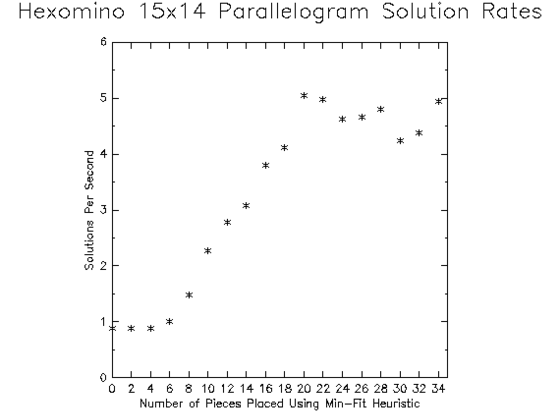
So I ran the solver against the 15x14 parallelogram initially applying the x heuristic, but switching to the min-fit heuristic when the number of remaining pieces hit some configured number. Unfortunately, an exhaustive examination of the search tree for this puzzle is not feasible. Instead, I used Monte-Carlo techniques to estimate the best time to stop using the x heuristic and start using the min-fit heuristic. Each data point shown in Figure 9 shows the average number of solutions found per second over 10,000 runs of the solver each initialized with a different random ordering of the nodes in each column of the DLX matrix. Each run was terminated the first time the 16th-to-last piece was removed from the puzzle. (In other words, once the 16th-to-last piece is placed, the solver examined all possible ways to place the last 15 pieces, but then terminates that run.) Solutions to this puzzle tend to appear in great bursts, and even at 10,000 runs I think there is quite a bit of uncertainty in these solution rates. It should also be noted that the DLX processing load for the early piece placements is enormous compared to the latter pieces. Terminating algorithm processing each time the 16th-to-last piece is removed means the great efforts expended to reduce the matrix were largely wasted. This results in reduced average performance.
Despite these weaknesses the analysis offers evidence that when there are more than approximately 20 pieces left to be placed in this puzzle, there is no real benefit to using the min-fit heuristic. In fact, using the min-fit heuristic beyond 20 pieces seems to show some slight degradation in performance; although the last data point (where the min-fit heuristic is used for the last 34 pieces placed) seems to again offer a performance increase. This could be a statistical fluke, but I rather suspect there is some significant benefit to filling the two opposite acute corners of the puzzle early. The x-heuristic simply ignores the tight corner at the opposite side of the puzzle. It is my suspicion that as puzzle sizes increase application of the min-fit heuristic across the entire puzzle will result in ever worsening performance relative to heuristics that (at least initially) pack confined regions of the puzzle first; but larger puzzles are exceedingly difficult to analyze even with Monte-Carlo techniques.
Depending on the geometry of the puzzle, it can be even more important to follow your intuition. Gerard's Polyomino Solution Page includes a puzzle similar to the one shown in Figure 10. This puzzle, however, is 2 squares longer and somewhat more difficult to solve. I was unable to find any solutions to this puzzle through exclusive use of the min-fit heuristic even after hours of execution time; but by initially picking the holes farthest from the geometric center of the puzzle (my "R" heuristic) and then switching to min-fit heuristic once the less-confined central cavity was reached I averaged about 9 solutions per minute over 6 hours of run time.
Most Constrained Hole (MCH) Algorithm
DLX is quite crafty, but all the linked list operations can be overly burdensome for small to medium sized puzzles. In a head-to-head match up, my implementation of de Bruijn's algorithm runs more than 6 times faster than DLX for the 10x6 pentomino puzzle (and remember — that's without the de Bruijn algorithm using the trick of placing the X piece first.) For the more complex three dimensional Tetris Cube puzzle, DLX fairs much better, but still takes more than twice as long to run as de Bruijn's algorithm.
The Most Constrained Hole (MCH) algorithm attempts to reap at least some of the benefits of DLX without incurring the high cost of its matrix manipulations.
I present this algorithm third, because the story flows better that way, but it is actually the first polycube solving algorithm I implemented and is of my own design. I make no claims of originality: it is a simple idea and others have independently devised similar algorithms. I first implemented a variant of this technique to solve pentomino puzzles one afternoon in the summer of 1997 whilst at a TCL/TK training class in San Jose, CA.
MCH simply chooses the hole that has the fewest number of fit possibilities as the next fill target. Therefore DLX (when using the min fit ordering heuristic) and MCH only deviate in their decision making process in those situations where a piece turns out to be more constrained than any hole. To find the MCH, the software examines each remaining hole in the puzzle, and for each of those holes it counts the number of ways the remaining pieces can be placed to fill that hole. The MCH is then taken to be the hole with the fewest fits.
Although DLX will sometimes choose a piece to place next rather than a hole to fill, the biggest difference between MCH and DLX is not in the step-by-step behavior of the two algorithms, but rather in their implementation. My polycube solving software has as one of its fundamental data structures an object called a GridPoint. During Puzzle initialization I create an array of GridPoint objects with the same dimensions as the Puzzle. So for the Tetris Cube I create a 4x4x4 matrix of GridPoints. To support MCH, at each GridPoint I create an array of 12 lists — one list for each of the twelve puzzle pieces. The list for piece B at GridPoint (3, 1, 2) contains all the images of piece B that fill the hole at grid coordinates (3, 1, 2). To count the total number of fits at (3, 1, 2) I traverse the image lists for all the pieces that have not yet been placed in the puzzle and count the total number that fit. To find the most constrained hole, I perform this operation at every open hole in the puzzle and take the hole with the minimum fit count.
Recall that for the de Bruijn algorithm a piece of size 6 with 24 unique rotations only requires 24 fit attempts, but that only works because the algorithm restricts itself to filling the hole with minimum coordinate values in z, y, x priority order. For MCH the image lists must contain all the images of a piece that fill a hole. So a piece with 6 cubelets and 24 unique rotations would have nominally 144 entries in the list. (I actually throw out images that don't fit inside the puzzle box as discussed in the section on image filters below.) So these lists can be rather long, and many lists at many holes have to be checked to find the MCH.
The whole idea sounds loopy I know, but for the case of the 10x6 pentomino puzzle, MCH runs 25% faster than DLX (which still makes it almost 5 times slower than de Bruijn). For the case of the Tetris Cube, MCH is the fastest of the three algorithms running about 2.5 times faster than DLX and about 10% faster than de Bruijn.
The solver also includes a variant of MCH that only considers those holes with the fewest number of neighboring holes. I call this estimated MCH (EMCH). This approach sometimes gets the true MCH wrong, but overall seems to perform better — about 25% faster for 10x6 Pentominoes and more than a third faster for the Tetris Cube.
I think for larger puzzles, when the number of images at each grid point starts to increase by orders of magnitude, this approach of explicit fit counting will break down. There are other ways you can estimate the MCH: I had one MCH variant that didn't count fits at all, but rather looked purely at the geometry of the open spaces near a hole to gauge how difficult it was going to be to fill. In any case, I only apply MCH on smaller 3-D puzzles because this is where I've found it to outpace the other two algorithms.
Combining the Algorithms
Each of the three algorithms examined had different strengths. When there are very few pieces, the simple de Bruijn algorithm had best performance. For medium sized 3-D puzzles, EMCH performed best. Only DLX can choose to iterate over all placements of a piece which can provide huge performance benefits in the right situation. (See, for example, the section on rotational redundancy constraint violations.) Also the ability to define different ordering heuristics makes DLX quite useful for large puzzles with non-trivial topologies.
To allow the best algorithm to be applied at the right time to the right problem, I've implemented all three algorithms into a single puzzle solving application with the capability to turn off one algorithm and turn on another when the number of remaining pieces reaches configured thresholds. As you shall see, this combined algorithmic approach gives much improved performance for many puzzles.
Software Optimizations
I still have the broad topic of constraints to discuss, but I first want to share some software optimizations I've made on the de Bruijn and MCH algorithms. Together these software optimizations reduced the time to find all Tetris Cube solutions with these algorithms by about a factor of five. (This probably just means my initial implementation was really bad, but I think the optimizations are still worth discussing.)
Bit Fields
I was originally tracking the occupancy state of the puzzle via a flag named occupied in each GridPoint object. To determine if an image fit in the puzzle, this flag was examined for each GridPoint used by the image. Most of the popular polyomino (e.g., Pentominoes) and polycube puzzles (e.g., Soma, Bedlam, Tetris) have an area or volume of not more than 64. This is rather convenient as it allows one to model the occupancy state of any of these puzzles with a 64-bit field. So I ditched all the occupied flags in the GridPoint array and replaced them all with a single 64 bit integer variable (named occupancyState) bound to the Puzzle as a whole. Each image object was similarly modified to store a 64-bit layoutMask identifying the GridPoints it occupies. To see if a particular image fits in the puzzle you now need only perform a binary-and of the puzzle's occupancyState with the image's layoutMask and check for a zero result. To place the piece, you need only perform the binary-or of the puzzle's occupancyState with the image's layoutMask and store that result as the new occupancyState. This is really greasy fast and cut the run times by more than a factor of two.
The only down-side to this approach is that it prevents you from solving puzzles that are larger than the size of the bit field. You could increase the size of the field, but this quickly starts to wipe out the benefit. But you can still take advantage of the performance benefit of bit masks for puzzles that are bigger than size 64 by simply using DLX until the total volume of remaining pieces is 64 or less. Then you can morph the data model into a bit-oriented form and use the MCH or de Bruijn algorithms to place the last several pieces (which is the only time speed really matters). For very large puzzles (e.g., a heptominoes puzzle) I think this approach will break down: by the time you get down to an area of size 64 the search tree is collapsing and it's probably too late for a data model morph to pay off.
Early MCH Fit Count Exit
The MCH routine examines different holes remaining in the puzzle and finds the number of possible fits for each of them. I modified the procedure that counts fits to simply return early once the number of fits surpasses the number of fits of the most constrained hole found so far. This trivial change sped the software up 20% for the Tetris Cube.
Fast Permutation Algorithm
In my original implementation of both MCH and de Bruijn's algorithm, I was lazily using an STL set (sorted binary tree) to store the index numbers of the remaining pieces. (Some of you are rudely laughing at me. Stop that.) Only the pieces in this set should be used to fill the next target hole. The index of the piece being processed is removed from the set. If the piece fits, the procedure recurses on itself starting with the now smaller set. Once all attempts to place a piece are exhausted, the piece is added back to the set, and the next entry in the set is removed and processed. This worked fine, but STL sets are not the fastest thing in the galaxy. As you might imagine there's been lots of research on fast permutation algorithms (dating back to the 17th century). I settled on an approach that was quite similar to what I was already doing, but the store for the list of free index numbers is a simple integer array instead of a binary tree. An index is "removed" from the array by swapping its position with the entry at the end of the array. So my STL set erase and insert operations were replaced with a pair of integer swaps. This change improved the fastest run times by about another 20%.
Constraints
The algorithms above observe the constraint that when a hole can't be fitted, or (in the case of DLX) a piece can't be fit they back up. But other constraints (beyond this obvious fit constraint) exist for polycube and polyomino puzzles which if violated prohibit solutions. My solver can take advantage of these constraints in two different ways. First I've implemented monitors that watch a particular constraint and when a violation is detected an immediate backtrack is triggered. Second, I've implemented a set of image filters that remove images that would violate constraints if used.
Backtrack Triggers
Let's first look at the technique of monitoring constraints during algorithm execution and triggering a backtrack when the constraint is violated.
Parity Constraint Violations
I first read about the notion of parity at Thorleif's SOMA page where in one of his Soma newsletters he references Jotun's proof. It's a simple idea: color each cube in the solution space either black or white in a three dimensional checkerboard pattern and then define the parity of the solution space to be the number of black cubes minus the number of white cubes. When you place a piece in the solution space, the number of black cubes it fills less the number of white cubes it fills is the parity of that image. Suppose that the parity for some image of a piece is 2. If you move that piece one position in any ordinal direction, all of its constituent cubes flip color and the parity of the piece will become -2. But those would be the only possible parities you could achieve with that piece: either 2 or -2. So the magnitude of the parity of a piece is defined by its shape, but depending where you place the piece, it could be either positive or negative.
As you place pieces, the total parity of all placed pieces takes a random walk away from an initial parity of zero, but to achieve a solution the random walk must end exactly at the parity of the solution space. It is possible for the random walk to get so far from the destination parity that it is no longer possible to walk back before you run out of pieces. More generally, you can get yourself in situations where it's just not possible to use the remaining pieces to walk back to exactly the right parity.
It is possible to show that some puzzles can't possibly be solved because the provided pieces have parities that just can't add up to the parity of the solution. As an example, consider again the 35 hexominoes shown in Figure 5. The total area of these pieces is 35x6 = 210. It is quite tempting to try to fit these pieces in a rectangular box. You could try boxes measuring 14x15, 10x21, 7x30, 6x35, 5x42 or even 3x70. The parity of all of these boxes is 0, so our random parity walk must end at 0. Of the 35 hexominoes 24 have parity 0 and the other 11 have parity magnitude 2. Because there is no way to take 11 steps of size 2 along a number line and end up back at 0, there is no way to fit the 35 hexominoes into any rectangular box.
Knowing that certain puzzles can't be solved without ever having to try to solve them is quite useful, but how can we make more general use of the parity constraints to speed up the search for solutions in puzzles?
Knuth attempted to enhance the performance of DLX though the use of parity constraints for the case of a one-sided hexiamond puzzle. The puzzle has four pieces with parity magnitude two (and the rest have parity zero). The puzzle as a whole has parity zero, so exactly two of these four pieces must be placed so their parity is -2 and two must be placed so their parity is 2. Knuth took the approach of dividing this problem into 6 subproblems, one for each way to choose the two pieces that will have positive parity. His expectation was that since each of the four pieces were constrained to have half as many images, that each subproblem would run 16 times as fast. Then, the total work for all 6 subproblems should be be only 6/16 of the work to solve the original (unconstrained) problem. But the total work to solve all 6 subproblems was actually more than the original problem. (I offer an explanation as to why this experiment failed below.)
I use a different approach to take advantage of parity constraints: simply monitor the parity of the remaining holes in the puzzle and if it ever reaches a value that the remaining pieces cannot achieve, then immediately trigger a backtrack.
To implement this parity-based backtracking feature, after each piece placement you must determine if the remaining puzzle pieces can be placed to achieve the parity of the remaining holes in the puzzle. This may sound computationally expensive, but it's not. Consider the Tetris Cube puzzle as an example. Piece A has parity 0, pieces B, E and L have a parity magnitude of 2, and the remaining eight pieces have a parity magnitude of 1. We can immediately forget about piece A since it has parity 0. So we have three pieces with parity magnitude 2 and eight pieces with parity magnitude 1. If you look at the parity of the pieces that are left at any given time, there are only (3+1) x (8+1) = 36 cases. During puzzle initialization I create a parity state object for each of these situations. So, for example, there is a parity state object that represents the specific case of having three remaining pieces of parity magnitude 1 and two remaining pieces of parity magnitude 2. In each of these 36 cases, I precalculate the parities that you can possibly achieve with that specific combination of pieces. I store these results in a boolean array inside the state object. So if you know your parity state, the task of determining if the parity of the remaining holes in the puzzle is achievable reduces to an array lookup. It looks something like this:
        if ( ! parityState->parityIsAchievable[parityOfRemainingHoles] )
            // force a backtrack due to parity violation
        else
            // parity looks ok so forge on
In addition to this boolean array, each parity state object also keeps track of its neighboring states in two arrays indexed by parity. One array is called place which you use to lookup your new state when a piece is placed; and the other is called unplace which you use to lookup your new state when a piece is removed. The only other task is to update the running sum of the parity of the remaining holes in the puzzle. So the processing for a piece placement looks like this:
        parityState = parityState->place[parityOfPiecePlaced];
        parityOfRemainigHoles -= parityOfPiecePlaced;
and piece removal processing looks like this:
        parityOfRemainigHoles += parityOfPieceRemoved;
        parityState = parityState->unplace[parityOfPieceRemoved];
Here, I'm using a double sided arrays so place[-2] and place[2] actually take you to the same state, saving the trouble of calculating the absolute value of parityOfPiecePlaced.
So the cost of parity checking is quite small, but typically parity violations do not start to appear until the last few pieces are being placed. In the 10x6 pentomino puzzle, the first parity violations did not appear until the 9th piece was placed; and adding the parity backtrack trigger to the fastest solver configuration for that puzzle actually increased run times by about 8%. (So adding just the above 5 lines of code to the de Bruijn processing loop increased the work to solve the problem by 1 part in 12! Indeed, even the time required to process the if statements that are used to see if various algorithm features are turned on, or if trace output is enabled, etc, measurably impairs the performance of the de Bruijn algorithm for this puzzle.) For the Tetris Cube, parity violations started to appear after only 6 pieces were placed, and use of the parity monitor improved performance by about 3%.
This parity backtrack trigger technique leaves the algorithms blinded to the true constraints on pieces with non-zero parity; so parity constraints are only hit haphazardly as opposed to being actively sought out by the algorithms. There is likely some better way to take advantage of the parity constraints on a puzzle. Thorleif found that for the case of the the Soma cube puzzle, forcibly placing pieces with non-zero parity first improved performance markedly; but I am skeptical that such an approach would work well in general because typically it's so much better to fill holes, rather than place pieces. One approach might be to simply assign some fractional weight to the counts maintained for piece columns that have non-zero parity. This would gently coax DLX into considering placing them earlier. I have not pursued such an investigation.
Still, with the right puzzle, monitoring parity constraints can be more useful. I've reproduced the box-in-a-diamond puzzle layout in Figure 11 to call attention to the parity of this puzzle. I designed this puzzle to have the the interesting property that its parity is exactly 22, which is the maximum parity the 35 hexomino puzzle pieces can possibly achieve. Any solution to this puzzle requires all eleven hexomino pieces with non-zero parity to favor black squares. Figure 12 shows one such solution with the 11 pieces having non zero parity highlighted. Monte Carlo estimation techniques showed that enabling the parity backtrack trigger on this puzzle produces about a two-thirds increase in performance. Although a substantial performance boost, this is less than I would have expected.
Volume Constraint Violations
The volume backtrack trigger, when enabled, performs the following processing after each piece placed:
- scans the open space of the puzzle, measuring the volume of each partition it finds, and
- triggers a backtrack if a volume is discovered that cannot be achieved by the remaining pieces.
To find and measure the volumes of subspaces in step 1, I use a simple fill algorithm. Step 2 of the problem — determining whether a particular volume is achievable — is easy if all pieces have the same size; but to handle the problem generally (when pieces are not all the same size) I use the same technique used by the parity monitor above: I precalculate the achievable volumes for each possible grouping of remaining pieces and track the group as a state variable.
The solver allows you to configure the minimum number of remaining pieces required to perform volume backtrack processing. As long as you turn off the volume backtrack feature sufficiently early, its cost is insignificant.
I originally implemented this backtrack trigger to keep DLX from partitioning polyomino puzzles into unfillable volumes while it wandered about the puzzle pursuing constrained holes or pieces; but I now believe it's often better to initially follow a simple packing strategy that precludes the creation of isolated volumes. I think this backtrack trigger may still be useful for some puzzles once the min-fit heuristic is enabled, but I have not had the time to study its effects.
Image Filters
In the previous sections we examined the technique of monitoring a constraint during algorithm execution and triggering a backtrack when the constraint is violated. Another (more aggressive) way you can take advantage of a constraint is to check all images one-by-one to see if using them would result in a constraint violation. For each image that causes a violation, simply remove it from the cache of available images. Some of the image filters discussed below are applied only once before the algorithms begin. Other image filers can be applied repeatedly (after each piece placement). In my solver, image filters can only be applied when DLX is active because the linked list structure of DLX makes it easy to remove and replace images at each algorithmic step.
Puzzle Bounds Constraint Violations
N.G. de Bruijn's original software used to solve the 10x6 pentomino problem predefined the layouts of the 12 puzzle pieces in each of their unique orientations. There are 63 unique orientations of the pieces in total, but the various possible translations of these orientations were not precalculated. This was a simple approach, and perhaps more importantly (in those days) made for a quite small program. This results, however, in the de Bruijn algorithm spending a lot of time checking fits for images that clearly fall outside the 10x6 box. These days, memory is cheap, so it is easy to improve on this basic approach. I've already explained the technique in the section on MCH above: for MCH I keep at each GridPoint a separate list for each piece which holds only those images of a piece that both fill the hole and actually fit in the puzzle box. I've done exactly the same thing for the de Bruijn algorithm: I created another array of image lists at each GridPoint, each list holding only the images of a particular piece that fill the hole with its root tiling node and also fit in the puzzle box. This completely eliminates all processing associated with placement attempts for images that don't even fit in the solution box.
By filtering out images that don't fit in the box, the average number of de Bruijn images at each hole in the 10x6 pentomino puzzle drops from 63 to 33.87 -- an almost 50% reduction. This should translate to a significant performance boost, though I can't say for sure since this is the only way I've ever implemented the algorithm.
Rotational Redundancy Constraint Violations
If you picked up a Tetris Cube when it was already solved; turned it on its side; and then excitedly told your brother you found a new solution, you'd likely get thumped. Because the puzzle box is cubic, there are actually 23 ways to rotate any solution to produce a new solution that is of the same shape as the original. My software can filter out solutions that are just rotated copies of previously discovered solutions (just enable the --unique command line option), but the search algorithms as described so far do actually find all 24 rotations of every solution (only to have 23 of them filtered out).
If by imperial decree, we only allow rotationally unique solutions, then it is possible to produce an image filter to take advantage of this constraint. If we simply fix the orientation of a piece that has 24 unique orientations, then the algorithms will only find rotationally unique solutions. Why does this work? If you fix the orientation of a piece, any solution you find is going to have that constrained piece in its fixed orientation; and the other 23 rotations of that same solution cannot possibly be found because those solutions have the constrained piece in some orientation that you never allowed to enter the box. Application of just this one filter reduced the time it takes DLX to find all solutions to the Tetris Cube from over seven hours down to about 20 minutes. Quite useful indeed.
It is possible to apply this same technique to puzzles that are not cubic; but instead of keeping the orientation of the piece completely fixed, you limit the set of rotations allowed.
But what if all of the pieces have fewer unique rotations than the puzzle has symmetric rotations? In this case you can also try constraining the translations of the piece within the solution box. This is slightly harder to do (it was for me anyway), and is not always guaranteed to eliminate all rotationally redundant solutions from the search. As an example try eliminating the rotationally redundant solutions from a 3x3x3 puzzle by constraining a puzzle piece that is a 1x1x1 cube. It can't be done. The best you can do is to constrain the piece to appear at one of four places: the center, the center of a face, the center of an edge and at a corner. This will eliminate some rotationally redundant solutions from the search, but not all.
A much harder problem is to try to eliminate rotationally redundant solutions from the search when none of the pieces in the puzzle have a unique shape. In this case, you can't simply constrain a single piece, but must instead somehow constrain in concert an entire set of pieces that share the same shape. I have some rough ideas on how one might algorithmically approach this problem, but I have not yet tried to work the problem out in detail.
For now, you can ask my solver to constrain any uniquely shaped piece so as to eliminate as many rotationally redundant solutions as possible. But even better, you can ask the solver to pick the piece to constrain. In this case it compares the results of constraining each uniquely shaped puzzle piece and picks the piece that will do the best job of eliminating rotationally redundant solutions. If two or more pieces tie, then it will pick the piece that after constraint has the fewest images that fit in the puzzle box. If for example you ask my solver to pick a piece for constraint on the 10x6 pentomino puzzle, it will pick X (the piece that looks like a plus sign), and constrain it so that it can only appear in the lower-left quadrant of the box. This is exactly the approach de Bruijn took when he solved the 10x6 pentomino puzzle 40 years ago, but de Bruijn identified this as the best constraint piece through manual analysis of the puzzle and programmed it as a special initial condition in his software. With my solver, you need only add the option -r to the command line.
Often times a piece that has been constrained will have so few remaining images that it becomes the best candidate for the first algorithm step. But of the algorithms I've implemented, only DLX will consider the option of iterating over the images of a single piece. So when running my solver with a piece constraint I usually use the DLX algorithm with a min-fit heuristic for at least the first piece placement. For the 10x6 pentomino problem, if you turn on constraint processing (which constrains the images of the X piece), but fail to use DLX for the first piece placement you'll find the run time to be eight times longer.
This feature was far and away the most difficult part of the solver for me to design and implement. (Perhaps some formal education in the field of spatial modeling would have been useful.) I have copious comments on the approach in the software. There are two parts to the problem: I first identify which rotations of the puzzle box as a whole produce a new puzzle box of exactly the same shape. This is normally a trivial problem, but the solver also handles situations where some of the puzzle pieces are loaded into fixed positions. If some of those pieces have a shape in common with pieces that are free to move about, then things get tricky. One-sided polyomino problems (which the solver also handles) also add complexity. Once I know the set of rotations that when applied to the puzzle can possibly result in a completely symmetric shape, I apply a second algorithm that filters the images produced for a (uniquely shaped) piece through a combination of rotational and/or translational constraints that eliminate these symmetries and has the net effect of preventing the algorithms from discovering rotationally redundant solutions. For a more exacting description of these techniques, please read my software comments for the methods Puzzle::initSymmetricRotationAndPermutationLists() and for Puzzle::genImageLists().
Parity Constraint Violations
You can also filter images based on parity constraints. So instead of waiting around for an image to be placed to trigger a parity backtrack; after each piece placement, you can look at the parity of each remaining image and determine if placing that image would introduce a parity violation; and if so, remove the image.
Of course I don't actually do the check for all images — only twice for each remaining piece with non-zero parity (once for positive parity and once for negative parity). If a violation would be introduced through the use of that piece when its parity is, say, negative, then I traverse the list of images for that piece and remove all the copies that have a negative parity. Also, the parity filter is skipped completely if the parity of the last piece placed was zero: nothing has changed in that case and it's pointless to look for new potential parity violations.
Applying the parity filter to the box-in-a-diamond puzzle causes the solver to filter out roughly half of the images of eleven pieces before DLX even starts. Replacing the parity backtrack trigger with the parity filter for this puzzle increased performance by more than 40%. In total, the solver running with the parity filter generates solutions 2.4 times as fast as it does without any parity constraint-based checks at all.
Volume Constraint Violations
You can also use volume constraints to filter images. This is very much akin to using volume constraints to trigger backtracks, but instead of waiting around for an image to be placed that partitions the open space; you can instead, one-by-one, place all remaining images in the puzzle and perform a volume check operation. This can be particularly useful as an initial step before you even set the algorithms to working. Of the 2056 images that fit in the 10x6 pentomino puzzle box, 128 of them are jammed up against a side or into a corner in such a way as to produce a little confined area that can't possibly be filled as seen in Figure 13. Searching for and eliminating these images up front improved my best run times for this puzzle by about 13%. This is the only technique I've found (other than the puzzle bounds filter discussed above) that actually improved performance for this classic puzzle.
The previous polyomino puzzles were all based on free polyominoes: polyomino pieces that you are free to not only rotate in the plane of the puzzle, but are also free to flip up side down; but there is another class of puzzles based on one-sided polyominoes: polyomino pieces that you are allowed to rotate within the plane, but are not allowed to flip up-side-down. Where there are only twelve free pentominoes, there are eighteen uniquely shaped one-sided pentominoes. Consider the problem of placing the eighteen one-sided pentominoes into a 30x3 box as shown in Figure 14. Because pieces can actually reach from one long wall of this puzzle box to the other, 40% of the images (776 out of 1936) that fit in this box produce unfillable volumes. (See Figure 15.) Applying the volume constraint filter to the images of this puzzle improved performance by about a factor of nine.
Consider next another puzzle I came across at Gerard's Polyomino Solution Page: placing the 108 free heptominoes into a 33x23 box with 3 symmetrically spaced holes left over as shown in Figure 16. One of the heptomino pieces has the shape of a doughnut with a corner bit out of it. This piece is shown in red in Figure 16. There's no way for another piece to fill this hole, so heptomino puzzles always leave at least one unfilled hole. To solve this puzzle, the doughnut piece clearly must be placed around one of these holes; but none of the algorithms are smart enough to take advantage of this constraint and will only place the doughnut around a hole by chance. And this could take a very long time indeed! Applying the volume constraint filter to this problem, removes not only the images that produce confined spaces around the perimeter of the puzzle, but also all images of the doughnut piece except those few that wrap one of the prescribed holes. The DLX min-fit heuristic will then correctly recognize the true inflexibility of this piece and place it first.
For 3-D puzzles, I think it would be rare for pieces to construct a planar barrier isolating two volumes large enough to cause serious trouble; accordingly, I have not studied the effects of this filter on 3-D puzzles.
In all of these examples I've only applied the volume filter once to the initial image set (prior to algorithm execution), but you can also apply the filter repeatedly, after each step in the algorithm (turning it off when the number of remaining pieces reaches some prescribed threshold). This should have the effect of giving DLX a better view of the puzzle constraints; but I haven't studied this primarily because my current implementation of the filter is so inefficient: at each algorithmic step each remaining image is temporarily placed and a graphical fill operation is performed to detect isolated volumes. This is simple, but the vast majority of these image checks are pointless. The next time I work on this project, I'll be improving the implementation of this filter which I hope will offer performance benefits when reapplied after each piece placement.
Fit Constraint Violations
Another filter I've implemented is based on a next-step fit constraint. By this I mean, if placing an image would result in either a hole that can't be filled, or a piece that can't be placed, then it is pointless to include that image in the image set. Running this fit filter on the 2056 images of the 10x6 pentomino puzzle finds all of the 128 images found by the volume constraint filter plus an additional 16 images like those shown in Figure 17. There can obviously be no puzzle solution with these piece placements. If the rotational redundancy filter is also enabled (which constrains the X piece to 8 possible positions in the lower left quadrant of the box), then the fit filter will eliminate 227 images. (There are numerous images that conflict with all of the constrained placements of the X piece.)
Note that running the fit filter twice on the same image set can sometimes filter additional images: on the first run you may remove images that were required for previously tested images to pass the fit check. If you run the fit filter twice on the 10x6 pentomino problem while the X piece is constrained, the number of filtered images jumps from 227 to 235. To do a thorough job you'd have to filter repeatedly until there was no change in the image set.
Although this filter is interesting, its current implementation is too slow to be of much practical use. I use DLX itself to identify fit-constraint violations and it takes 45 seconds to perform just the first fit filtering operation for the box-in-a-diamond hexomino puzzle on my 2.5 GHz P4. I suspect I could write something that does the same job much quicker, but I'm skeptical I could make it fast enough to be effective. Still, if your aim is the lofty goal of finding all solutions to this puzzle, this filter could prove worth-while: 45 seconds is nothing for at least the first several piece placements of this sizable puzzle.
Image Filter Performance (or lack thereof)
Some of the image filters discussed above are only run once before the algorithms begin. I wanted to share some insight as to why such filters sometimes don't give the performance gains you might expect.
As a first example, consider the effects of filtering pentominoes images that fall outside the 10x6 puzzle box. This cuts the total number of images that have to be examined by the de Bruijn algorithm at each algorithm step by almost a factor 2. In an extraordinary flash of illogic, you might conclude that since there are 12 puzzle pieces, the performance advantage to the algorithm would be a factor of 212 = 4096. The problem with this logic is that the algorithm immediately skips these images as soon as they are considered for placement anyway.
For the same reason, filtering images that produce volume constraint violations before you begin running the algorithms do not give such exponential performance gains: such images typically construct tiny little confined spaces that the algorithm would have quickly identified as unfillable anyway.
But the filter that removes images of a single piece to eliminate rotational redundancies among discovered solutions seems different: the images removed are not images that will necessarily cause the algorithm to immediately backtrack and so you might reasonably expect the filter to not only reduce the number of solutions found for the Tetris Cube by a factor of 24 (which it does); but also to improve the overall performance of the algorithm by a factor of 24, but it only gave a factor of 21. (Close!)
Knuth expected that reducing the number of images of 4 pieces each by a factor of 2 (to take advantage of a parity constraint on a one-sided hexiamond puzzle) would lead to a reduction in the work needed to solve the puzzle by a factor of 16, but the gains again fell far short of this expectation.
And although I wasn't expecting a performance improvement factor of 211 from the parity filter for the box-in-a-diamond problem, I thought I'd get a lot more than a factor of 2.4 (which is all it gave me). This result was very surprising to me.
The problem in all of these cases is that you're trying to extract efficiencies from a search tree that is already significantly pruned by the algorithm. Here are some other observations that might be illuminating.
First, consider the case where you a priori force a piece whose images are to be filtered to be placed first; and then reduce the number of images of that piece by a factor of N. Then the number of ways to place that first piece is reduced by a factor of N. Assuming each of those placements originally had similar work loads, then the total work would indeed be reduced by a factor of N. But what if you always placed this piece last? Would performance still improve by a factor of N? Of course not! The vast majority of search paths terminate in failure before you even get to the last piece. Now assuming the piece is not being placed first, or last but is instead placed uniformly across the search tree, you'll find that a sizable percentage of search paths don't even use the filtered piece: they die off before that piece can be placed. Filtering the images of that piece won't reduce the weight from these branches of the search tree at all.
Second, the vast majority of the appearances of the piece will be high up in the branches of the search tree. At this part of the tree, the branching factor is small and obviously drops below 1 at some point. Because of this, when you prune the tree at one of the appearances of the constraint piece, you can't assume that the weight of the path left behind is negligible (even though that weight is shared by other paths).
These arguments are obviously imprecise and contain (at least) one serious flaw: the DLX algorithm (unlike the other two) can reshape the entire search tree after you constrain the piece to take advantage of its new constrained nature, but if during execution of the algorithm, the piece is still found to be less constrained than other elements of the puzzle, then the arguments above still apply. Even if DLX decides to place the newly constrained piece first (and it often does), the average branching factor will still not typically improve sufficiently to achieve a factor of N performance improvement.
Performance Comparisons
Table 2 shows the performance results for a few different puzzles with many different combinations of algorithms, backtrack triggers and image filters. Many of these results have already been discussed in earlier sections but are provided here in detail. The run producing the best unique solution production rate is highlighted in yellow for each puzzle. The table key explains everything.
Using the unique solution generation rate as a means of comparing algorithm quality is flawed as these rates are not completely consistent from run-to-run. The relative performance of the different algorithms can also change with the processor design because, for example, one algorithm may make better use of a larger instruction or data cache. I liked Knuth's technique of simply counting linked list updates to measure performance, but since I'm comparing different algorithms, such an approach seems difficult to apply.
| Test Case | Algorithms | Image Filters | Backtrack Triggers | Monte-Carlo | Attempts | Fits | Unique | Run Time (hh:mm:ss) | Rate | |||||||||
|---|---|---|---|---|---|---|---|---|---|---|---|---|---|---|---|---|---|---|
| DLX | MCH | EMCH | de Bruijn | R | P | V | F | P | V | N | R | S | ||||||
| P-1 | 12f | 0 | 0 | 0 | OFF | OFF | OFF | OFF | OFF | OFF | - | - | - | 3,615,971 |
3,615,971 |
2339 |
00:00:38.761 | 60 |
| P-2 | 0 | 12 | 0 | 0 | OFF | OFF | OFF | OFF | OFF | OFF | - | - | - | 138,791,760 |
9,077,194 |
2339 |
00:00:29.250 | 80 |
| P-3 | 0 | 0 | 12 | 0 | OFF | OFF | OFF | OFF | OFF | OFF | - | - | - | 191,960,438 |
12,114,615 |
2339 |
00:00:22.485 | 104 |
| P-4 | 0 | 0 | 0 | 12 | OFF | OFF | OFF | OFF | OFF | OFF | - | - | - | 178,983,597 |
25,848,915 |
2339 |
00:00:06.086 | 384 |
| P-5 | 12f | 0 | 0 | 0 | ON | OFF | OFF | OFF | OFF | OFF | - | - | - | 892,247 |
892,247 |
2339 |
00:00:09.449 | 246 |
| P-6 | 0 | 12 | 0 | 0 | ON | OFF | OFF | OFF | OFF | OFF | - | - | - | 114,753,421 |
7,646,476 |
2339 |
00:00:24.504 | 95 |
| P-7 | 0 | 0 | 12 | 0 | ON | OFF | OFF | OFF | OFF | OFF | - | - | - | 153,036,807 |
9,875,973 |
2339 |
00:00:19.992 | 117 |
| P-8 | 0 | 0 | 0 | 12 | ON | OFF | OFF | OFF | OFF | OFF | - | - | - | 133,086,329 |
20,073,791 |
2339 |
00:00:04.700 | 498 |
| P-9 | 12f | 11 | 0 | 0 | ON | OFF | OFF | OFF | OFF | OFF | - | - | - | 12,411,752 |
924,167 |
2339 |
00:00:02.701 | 866 |
| P-10 | 12f | 0 | 11 | 0 | ON | OFF | OFF | OFF | OFF | OFF | - | - | - | 20,374,275 |
1,425,356 |
2339 |
00:00:02.569 | 911 |
| P-11 | 12f | 0 | 0 | 11 | ON | OFF | OFF | OFF | OFF | OFF | - | - | - | 17,703,679 |
2,455,947 |
2339 |
00:00:00.579 | 4049 |
| P-12 | 12f | 0 | 0 | 11 | ON | OFF | OFF | OFF | ON | OFF | - | - | - | 17,572,247 |
2,454,746 |
2339 |
00:00:00.620 | 3781 |
| P-13 | 12f | 0 | 0 | 11 | ON | OFF | 12 | OFF | OFF | OFF | - | - | - | 15,198,004 |
2,091,215 |
2339 |
00:00:00.510 | 4592 |
| OP-1 | 18f | 0 | 0 | 12 | ON | OFF | OFF | OFF | OFF | OFF | - | - | - | 38,479,316 |
7,060,175 |
46 |
00:00:03.611 | 12.7 |
| OP-2 | 18f | 0 | 0 | 12 | ON | OFF | 18 | OFF | OFF | OFF | - | - | - | 1,930,304 |
668,117 |
46 |
00:00:00.411 | 112.1 |
| TC-1 | 12f | 0 | 0 | 0 | OFF | OFF | OFF | OFF | OFF | OFF | - | - | - | 1,502,932,134 |
1,502,932,134 |
9839 |
07:21:31 | 0.37 |
| TC-2 | 0 | 12 | 0 | 0 | OFF | OFF | OFF | OFF | OFF | OFF | - | - | - | 58,306,235,943 |
1,604,152,199 |
9839 |
02:54:07 | 0.94 |
| TC-3 | 0 | 0 | 12 | 0 | OFF | OFF | OFF | OFF | OFF | OFF | - | - | - | 109,746,141,977 |
2,835,090,958 |
9839 |
02:19:27 | 1.18 |
| TC-4 | 0 | 0 | 0 | 12 | OFF | OFF | OFF | OFF | OFF | OFF | - | - | - | 737,892,116,733 |
38,637,085,619 |
9839 |
03:29:26 | 0.78 |
| TC-5 | 12f | 0 | 0 | 0 | ON | OFF | OFF | OFF | OFF | OFF | - | - | - | 68,141,081 |
68,141,081 |
9839 |
00:20:37 | 7.95 |
| TC-6 | 0 | 12 | 0 | 0 | ON | OFF | OFF | OFF | OFF | OFF | - | - | - | 9,727,894,584 |
297,896,605 |
9839 |
00:33:17 | 4.93 |
| TC-7 | 0 | 0 | 12 | 0 | ON | OFF | OFF | OFF | OFF | OFF | - | - | - | 19,436,156,238 |
551,894,232 |
9839 |
00:28:45 | 5.70 |
| TC-8 | 0 | 0 | 0 | 12 | ON | OFF | OFF | OFF | OFF | OFF | - | - | - | 140,658,669,459 |
7,992,209,655 |
9839 |
00:43:08 | 3.80 |
| TC-9 | 12f | 11 | 0 | 0 | ON | OFF | OFF | OFF | OFF | OFF | - | - | - | 2,153,543,323 |
72,670,225 |
9839 |
00:07:20 | 22.35 |
| TC-10 | 12f | 0 | 11 | 0 | ON | OFF | OFF | OFF | OFF | OFF | - | - | - | 4,196,219,275 |
129,746,342 |
9839 |
00:06:02 | 27.16 |
| TC-11 | 12f | 0 | 0 | 11 | ON | OFF | OFF | OFF | OFF | OFF | - | - | - | 32,810,876,767 |
1,898,921,763 |
9839 |
00:09:48 | 16.74 |
| TC-12 | 12f | 11 | 6 | 4 | ON | OFF | OFF | OFF | OFF | OFF | - | - | - | 10,380,361,756 |
453,289,747 |
9839 |
00:04:04 | 40.25 |
| TC-13 | 12f | 11 | 6 | 4 | ON | OFF | OFF | OFF | ON | OFF | - | - | - | 9,421,945,256 |
439,737,621 |
9839 |
00:03:57 | 41.53 |
| HP-1 | 35x 0f | 0 | 0 | 0 | ON | OFF | OFF | OFF | OFF | OFF | 10,000 |
16 |
5 |
1,131,766,165 |
1,131,766,165 |
17,435 |
05:28:15 | 0.885 |
| HP-2 | 35x 2f | 0 | 0 | 0 | ON | OFF | OFF | OFF | OFF | OFF | 10,000 |
16 |
5 |
1,131,686,519 |
1,131,686,519 |
17,435 |
05:29:15 | 0.883 |
| HP-3 | 35x 4f | 0 | 0 | 0 | ON | OFF | OFF | OFF | OFF | OFF | 10,000 |
16 |
5 |
1,097,629,194 |
1,097,629,194 |
17,435 |
05:28:58 | 0.883 |
| HP-4 | 35x 6f | 0 | 0 | 0 | ON | OFF | OFF | OFF | OFF | OFF | 10,000 |
16 |
5 |
849,818,771 |
849,818,771 |
17,435 |
04:48:02 | 1.009 |
| HP-5 | 35x 8f | 0 | 0 | 0 | ON | OFF | OFF | OFF | OFF | OFF | 10,000 |
16 |
5 |
507,044,709 |
507,044,709 |
17,435 |
03:14:58 | 1.490 |
| HP-6 | 35x 10f | 0 | 0 | 0 | ON | OFF | OFF | OFF | OFF | OFF | 10,000 |
16 |
5 |
326,708,081 |
326,708,081 |
17,435 |
02:07:31 | 2.279 |
| HP-7 | 35x 12f | 0 | 0 | 0 | ON | OFF | OFF | OFF | OFF | OFF | 10,000 |
16 |
5 |
272,000,566 |
272,000,566 |
17,435 |
01:44:36 | 2.778 |
| HP-8 | 35x 14f | 0 | 0 | 0 | ON | OFF | OFF | OFF | OFF | OFF | 10,000 |
16 |
5 |
241,487,173 |
241,487,173 |
17,435 |
01:34:34 | 3.073 |
| HP-9 | 35x 16f | 0 | 0 | 0 | ON | OFF | OFF | OFF | OFF | OFF | 10,000 |
16 |
5 |
420,363,728 |
420,363,728 |
30,945 |
02:15:46 | 3.799 |
| HP-10 | 35x 18f | 0 | 0 | 0 | ON | OFF | OFF | OFF | OFF | OFF | 10,000 |
16 |
5 |
880,638,007 |
880,638,007 |
60,415 |
04:04:34 | 4.117 |
| HP-11 | 35x 20f | 0 | 0 | 0 | ON | OFF | OFF | OFF | OFF | OFF | 10,000 |
16 |
5 |
1,363,568,660 |
1,363,568,660 |
106,960 |
05:53:36 | 5.041 |
| HP-12 | 35x 22f | 0 | 0 | 0 | ON | OFF | OFF | OFF | OFF | OFF | 10,000 |
16 |
5 |
1,508,462,348 |
1,508,462,348 |
112,975 |
06:18:54 | 4.970 |
| HP-13 | 35x 24f | 0 | 0 | 0 | ON | OFF | OFF | OFF | OFF | OFF | 10,000 |
16 |
5 |
1,728,349,705 |
1,728,349,705 |
119,370 |
07:10:09 | 4.625 |
| HP-14 | 35x 26f | 0 | 0 | 0 | ON | OFF | OFF | OFF | OFF | OFF | 10,000 |
16 |
5 |
1,718,965,943 |
1,718,965,943 |
119,862 |
07:09:28 | 4.652 |
| HP-15 | 35x 28f | 0 | 0 | 0 | ON | OFF | OFF | OFF | OFF | OFF | 10,000 |
16 |
5 |
1,858,118,645 |
1,858,118,645 |
133,872 |
07:44:54 | 4.799 |
| HP-16 | 35x 30f | 0 | 0 | 0 | ON | OFF | OFF | OFF | OFF | OFF | 10,000 |
16 |
5 |
1,700,793,486 |
1,700,793,486 |
108,882 |
07:07:56 | 4.241 |
| HP-17 | 35x 32f | 0 | 0 | 0 | ON | OFF | OFF | OFF | OFF | OFF | 10,000 |
16 |
5 |
1,735,853,837 |
1,735,853,837 |
115,466 |
07:19:01 | 4.384 |
| HP-18 | 35x 34f | 0 | 0 | 0 | ON | OFF | OFF | OFF | OFF | OFF | 10,000 |
16 |
5 |
1,912,535,104 |
1,912,535,104 |
140,085 |
07:53:32 | 4.930 |
| HBD-1 | 35f | 0 | 0 | 0 | OFF | OFF | OFF | OFF | OFF | OFF | 10,000 |
22 |
0 |
9,381,994,687 |
9,381,994,687 |
16,735 |
49:54:40 | 0.093 |
| HBD-2 | 35a@160 15f | 0 | 0 | 0 | OFF | OFF | OFF | OFF | OFF | OFF | 10,000 |
22 |
0 |
978,785,202 |
978,785,202 |
3731 |
05:28:58 | 0.189 |
| HBD-3 | 35a@160 15f | 0 | 0 | 0 | OFF | OFF | OFF | OFF | ON | OFF | 10,000 |
22 |
0 |
968,436,589 |
968,436,589 |
5761 |
05:08:05 | 0.312 |
| HBD-4 | 35a@160 15f | 0 | 0 | 0 | OFF | 35 | OFF | OFF | OFF | OFF | 10,000 |
22 |
0 |
1,156,373,212 |
1,156,373,212 |
8738 |
05:27:04 | 0.445 |
| HBD-5 | 35a@160 15f | 0 | 0 | 0 | OFF | 35 | 35 | OFF | OFF | OFF | 10,000 |
22 |
0 |
1,629,292,460 |
629,292,460 |
5652 |
02:44:54 | 1.582 |
| KEY | |||
|---|---|---|---|
| Test Case | P | Pentomino 10x6 | Test Cases P, OP, and TC were run on a 2.5 GHz P4 running Unbuntu Linux. Test Cases HP and HBD were run on a 2.4 GHz Core 2 Quad CPU Q6600 running Windows XP (using only one of the four processors). |
| OP | One-Sided Pentomino 30x3 | ||
| TC | Tetris Cube | ||
| HP | Hexomino 15x14 Parallelogram | ||
| HBD | Hexomino Box-in-a-Diamond | ||
| Algorithms | The number in each algorithm column is the number of remaining pieces when the algorithm is activated. For the case of DLX multiple activation numbers can be given, each with a different ordering heuristic. An entry 12f means the min-fit ordering heuristic is activated when 12 pieces remain. Other heuristics used are the x heuristic which picks the hole with minimum x coordinate value; and the a@160 heuristic which picks the hole that forms the minimum angle from the center of the puzzle with an initial angle of 160 degrees. | ||
| Image Filters | R | Rotational Redundancy Filter | A number in a column gives the minimum number of remaining pieces for the image filter to be applied. |
| P | Parity Constraint Filter | ||
| V | Volume Constraint Filter | ||
| F | Fit Constraint Filter | ||
| Backtrack Triggers | P | Parity Constraint Backtrack Trigger | A number in a column gives the minimum number of remaining pieces for the backtrack trigger to be applied. |
| V | Volume Constraint Backtrack Trigger | ||
| Monte-Carlo | N | Number of trials. | |
| R | If after removing a piece from the puzzle there are exactly R pieces left to place, the Monte-Carlo trial is ended. | ||
| S | Seed value to the Mersene Twister random number generator. | ||
| Attempts | The number of times pieces were attempted to be placed. | ||
| Fits | The number of times pieces were successfully placed. | ||
| Unique | The number of unique solutions found. | ||
| Run Time | The total run time for the test. | ||
| Rate | The number of unique solutions found per second (Unique / Run Time). | ||
Test Case P: Pentominoes in a 10x6 Box
The first set of test cases (P) examines the 10x6 pentomino puzzle shown in Figure 3. Runs 1 through 4 show the performance of the four basic algorithms.
Comparing these first four runs with runs 5 through 8 shows the significant performance advantage of the rotational redundancy filter. This filter consistently offers significant performance gains when looking for all solutions to a symmetric puzzle. Also note that DLX performs relatively better with this filter enabled as it's the only algorithm capable of iterating over the possible placements of the piece constrained by the filter.
Runs 9 through 11 use DLX only for the first piece placement (to take full advantage of the rotational redundancy filter) but then switch to the other lighter-weight algorithms to place the last 11 pieces. Comparing run 8 with run 11 shows this combined algorithmic approach to be about eight times faster than any single algorithm.
Run 12 shows that although the parity filter does offer a very moderate reduction in attempts and fits, the net effect is a reduction in the production rate of unique solutions.
Run 13 uses a one-shot volume filter to expunge many useless images from the image set and results in about a 13% increase in performance.
Test Case OP: One-sided Pentominoes in a 30x3 Box
The second set of test cases (OP) examines the problem of placing the one-sided pentominoes in a 30x3 box as shown in Figure 14. The volume filter is shown to be particularly useful for this puzzle delivering a factor-of-nine performance improvement.
Test Case TC: Tetris Cube
The third set of test cases (TC) examines the Tetris Cube as shown in Figure 1. The first four runs show the performance of MCH and EMCH to be superior to DLX and de Bruijn for this small 3-D puzzle.
Runs 5 through 8 again show the huge performance benefits of the rotational redundancy filter; and again DLX performs relatively better than the other algorithms with the rotational redundancy filter active, even outperforming de Bruijn for this 3D puzzle.
In runs 9 through 11 I start to combine the algorithms only using DLX to place the first piece (to get it to iterate over the possible placements of the piece constrained by the rotational redundancy filter) but then switching to just one of the simpler algorithms. As can be seen from the table, the benefits of this combined approach are quite significant.
In run 12 all four algorithms are combined to solve the puzzle. If you number pieces as you place them in the box counting down from 12 (so the last piece placed is numbered 1); then DLX was used to place piece 12; MCH to place pieces 11 through 7; EMCH to place pieces 6 and 5; and de Bruijn was used to place pieces 4 through 1. As the number of remaining pieces gets smaller, it pays to use simpler algorithms. Compare the performance of run 12 with the performance of runs 5 through 8 (where just one algorithm was used) and you see that the combined algorithmic approach is more than 5 times faster than the fastest of those single algorithm runs.
Run 13 shows that the parity backtrack trigger offers a small benefit (about 3%) for this puzzle. It is interesting that run 13 is well over 100 times faster than the straight DLX approach used in run 1.
Test Case HP: Hexominoes in a 15x14 Parallelogram
The fourth set of test cases (HP) examines the problem of placing the 35 hexominoes in the 15x14 parallelogram shown in Figure 6. Here I did not try to find the overall best solver configuration, but instead only studied the effects of packing pieces simply from left to right (using the x ordering heuristic) for initial piece placements and then switching to the DLX min-fit heuristic for latter piece placements. I should not have had the rotational redundancy filter active for these tests — this only slows solution production rates when examining such a small portion of the search tree — but I didn't want to tie up my computer for another week to rerun the tests. The best performance was had when using the min-fit heuristic only for the last twenty piece placements. Using the min-fit heuristic for more than twenty pieces resulted in little performance change but seems to exhibit some small degradation.
It is likely that application of the volume constraint filter, the parity constraint backtrack trigger, and the de Bruijn algorithm (for latter piece placements) would offer additional performance gains for this puzzle.
Test Case HBD: Hexominoes Box-in-a-Diamond
The last set of test cases (HBD) examines the hexomino box-in-a-diamond puzzle shown in Figure 12. The first run is a straight no-frills DLX run using the min-fit heuristic. For the second run I instead used my angular ordering heuristic which packs pieces into the puzzle in a counter clock-wise direction. I started placing pieces at 160 degrees (about ten o-clock) so that the less confined region at the top of the puzzle would be left for last. Once there were only 15 pieces left I switched to the min-fit heuristic. The number 15 was just a guess and probably too low for best performance; but this approach was still twice as fast as using a pure min-fit heuristic.
Run 3 shows that enabling the parity constraint backtrack trigger improved performance by about 65% in this very high-parity puzzle. Run 4 switches to the parity constraint filter which improves performance by another 42%.
Most interestingly, Run 5 shows a one-shot application of the volume constraint filter increased performance by a factor of 3.5.
Software
This software is protected by the GNU General Public License (GPL) Version 3. See the README.txt file included in the zip file download for more information.
EDIT (February 11, 2019): the software described and linked below is several years old, but is retained here as it is consistent with this document. I encourage you, however, to instead download and use my improved version of polycube linked from my more recent article on FILA.
Download
- README.txt (copyright, build and run instructions)
- RELEASE_NOTES.txt (summary of changes for each release)
- polycube.exe (polycube solver executable for Windows)
- tetriscube_def.txt (definition file for the Tetris Cube puzzle)
- bedlamcube_def.txt (definition file for the Bedlam Cube puzzle)
- somacube_def.txt (definition file for the Soma Cube puzzle)
- Several definitions for the Pentominoes puzzle for solutions of different shapes.
- Puzzle solver C++ source
The source is about 10,000 lines of C++ code, with dependencies on two other libraries (boost and the Mersene Twister random number generator) which are also included in the download. The executable file polycube.exe is a Windows console application (sorry, no GUIs folks). For non-Windows platforms you'll need to compile the source.
Running the Software
The README.txt file gives the full details about how to run the software (algorithm control, solution output control, trace output control, puzzle definition file formats, etc); but here is a brief introduction. Simply pass polycube one (or more) puzzle definition files on the command like this:
polycube def/pentominoes_10x6_def.txt
This will immediately start spitting out solutions to the 10x6 pentominoes puzzle. Once you see that it's working you'll probably want to explore available command line options. To see them run:
polycube --help
There are several puzzle definition files provided. These are simple text files that look like this:
# Tetris Cube Puzzle Definition
D:xDim=4:yDim=4:zDim=4
C:name=A:type=M:layout=0 0 2,  1 0 2,  2 0 2,  2 0 1,  2 0 0,  2 1 0  # Blue angle with end-notch
C:name=B:type=M:layout=0 0 0,  1 0 0,  2 0 0,  2 1 0,  2 2 0,  2 1 1  # Blue angle with mid-notch
C:name=C:type=M:layout=0 0 0,  1 0 0,  1 0 1,  2 0 1,  2 1 1          # Blue angled staircase
C:name=D:type=M:layout=0 0 0,  1 0 0,  2 0 0,  2 1 0,  3 1 0          # Blue 2-D serpent
C:name=E:type=M:layout=0 0 1,  0 0 0,  1 0 0,  1 1 0,  1 2 0,  2 1 0  # Red dog with tail
C:name=F:type=M:layout=0 0 0,  1 0 0,  0 0 1,  1 0 1,  0 1 0          # Red ziggurat
C:name=G:type=M:layout=0 2 0,  0 1 0,  0 0 0,  1 0 0,  2 0 0          # Red angle
C:name=H:type=M:layout=0 0 0,  1 0 0,  2 0 0,  3 0 0,  2 1 0          # Red line with mid-notch
C:name=I:type=M:layout=0 0 1,  1 0 1,  2 0 1,  0 1 1,  0 1 0          # Yellow pole with twisty top
C:name=J:type=M:layout=0 0 0,  1 0 0,  1 0 1,  1 1 1,  2 1 1          # Yellow cork-screw
C:name=K:type=M:layout=0 0 0,  1 0 0,  2 0 0,  1 1 0,  1 1 1          # Yellow radar dish
C:name=L:type=M:layout=0 1 0,  1 1 0,  1 1 1,  2 1 1,  1 0 1,  1 2 1  # Yellow sphinx
~D
The type=M means the piece is mobile and free to move about (the typical case), but you can also declare a piece to be type S (stationary) to forcibly load the piece at the given coordinates. It's often easier to define the puzzle pieces graphically. Here's a definition file for the box-in-a-diamond hexomino puzzle that uses graphical layouts for piece definitions.
# Box-in-a-Diamond Hexomino Puzzle Definition
D:xDim=23:yDim=23:zDim=1
L
. . . . . . . . . . . A . . . . . . . . . . . . . . . . . . . . . . . . . . .
. . . . . . . . . . . A . B B . C . . D . . . E . . F . . . . . . . . . . . .
. . . . . . . . . . . A . B . . C C . D . . E E . . F . . . . . . . . . . . .
. . . . . . . . . . . A . B . . C . . D D . E . . F F . . . . . . . . . . . .
. . . . . . . . . . . A . B . . C . . D . . E . . F . . . . . . . . . . . . .
. . . . . . . . . . . A . B . . C . . D . . E . . F . . . . . . . . . . . . .
. . . . . . . . . . . . . . . . . . . . . . . . . . . . . . . . . . . . . . .
. G G . H H . I I . J . . K . . . L . M M M . N . . . O . . . P . . . Q . . .
. G G . H . . I . . J J . K K . L L . M . . . N N N . O . . . P . . . Q . . .
. G . . H H . I . . J J . K K . L . . M . . . N . . . O O O . P P . . Q Q Q .
. G . . H . . I I . J . . . K . L L . M . . . N . . . . O . . . P P . . . Q .
. . . . . . . . . . . . . . . . . . . . . . . . . . . . . . . . . . . . . . .
R . . . S . . . T . . . U U U . V V . . W W . . X X . . . Y . . . Z . . 1 . .
R R R . S S . . T T . . . U . . . V V . . W . . . X . . Y Y Y . Z Z . . 1 1 .
. R . . . S S . . T . . . U . . . V . . . W W . . X . . . Y . . . Z Z . . 1 1
. R . . . S . . . T T . . U . . . V . . . W . . . X X . . Y . . . Z . . . . 1
. . . . . . . . . . . . . . . . . . . . . . . . . . . . . . . . . . . . . . .
. . . . . 2 2 . 3 . . . 4 . . . 5 . . . 6 . . . 7 7 . . 8 8 . . 9 9 . . . . .
. . . . . 2 2 . 3 3 3 . 4 4 . . 5 5 5 . 6 . 6 . 7 7 7 . 8 8 . . . 9 9 . . . .
. . . . . 2 2 . 3 3 . . 4 4 4 . 5 . 5 . 6 6 6 . . 7 . . . 8 8 . 9 9 . . . . .
~L
L:stationary=*
* * * * * * * * * * * . * * * * * * * * * * *
* * * * * * * * * * . . . * * * * * * * * * *
* * * * * * * * * . . . . . * * * * * * * * *
* * * * * * * * . . . . . . . * * * * * * * *
* * * * * * * . . . . . . . . . * * * * * * *
* * * * * * . . . . . . . . . . . * * * * * *
* * * * * . . . . . . . . . . . . . * * * * *
* * * * . . . . . . . . . . . . . . . * * * *
* * * . . . . . . . . . . . . . . . . . * * *
* * . . . . * * * * * * * * * * * . . . . * *
* . . . . . * * * * * * * * * * * . . . . . *
. . . . . . * * * * * * * * * * * . . . . . .
* . . . . . * * * * * * * * * * * . . . . . *
* * . . . . * * * * * * * * * * * . . . . * *
* * * . . . . . . . . . . . . . . . . . * * *
* * * * . . . . . . . . . . . . . . . * * * *
* * * * * . . . . . . . . . . . . . * * * * *
* * * * * * . . . . . . . . . . . * * * * * *
* * * * * * * . . . . . . . . . * * * * * * *
* * * * * * * * . . . . . . . * * * * * * * *
* * * * * * * * * . . . . . * * * * * * * * *
* * * * * * * * * * . . . * * * * * * * * * *
* * * * * * * * * * * . * * * * * * * * * * *
~L
~D
Note that a single stationary piece named * is used to shape the puzzle.
Planned Features
When I get time to work on this again, these are the features I'll be adding:
- Improve the implementation of the volume constraint filter. This filter often offers remarkable performance enhancements, but I think I can make it faster and increase the range of problems where it is effective.
- Extend the rotational symmetry filter to also detect and filter 3-D reflective symmetries. This is exactly like one-sided polyomino constraints: one-sided polyomino pieces are free to rotate in 2 dimensions but not in 3; but because every polyomino piece has a mirror that's also in the piece set, constructions that have mirror symmetries can be flipped up-side-down (a 180 degree rotation through the third dimension) to produce a new valid solution. Similarly, all 3-D puzzles are effectively one-sided relative to the 4th dimension: we puny humans cannot take a puzzle piece and rotate it 180 degrees through the 4th dimension. If we could, we could transform any piece into its mirror image. But, if the piece set as a whole is complete (again, in the sense that the mirror of every piece is also in the available piece set); then it is possible to rotate any solution to any puzzle having mirror symmetries 180 degrees through the 4th dimension to produce a new valid solution. I think it should be straight-forward to further constrain the allowed rotations and/or translations of a piece to eliminate such trivial solutions from the search and achieve additional performance gains for those puzzles that have this property. (E.g., any soma cube or pentacube construction with mirror symmetries should be able to take advantage this technique.)
- Add support for multi-threading and/or distributed processing.
- Add support for graphical rendering of puzzle trace and solution output.
- Additional constraint-based image filters and/or backtrack triggers.
- Possibly add other algorithms.
Solutions
Here are all the solutions to the Tetris Cube and a few other popular puzzles:
- bedlamcube_out.txt (all 19186 solutions to the Bedlam Cube puzzle)
- pentominoes_10x6_out.txt (all 2339 solutions to the 10x6 pentomino puzzle)
- pentominoes_onesided_30x3_out.txt (all 46 solutions to the 30x3 one-sided pentomino puzzle)
- somacube_out.txt (all 480 solutions to the Soma Cube puzzle)
- tetriscube_out.txt (all 9839 solutions to the Tetris Cube puzzle)
The solutions for 3-D puzzles need explanation. The first three solutions to the Tetris Cube are shown below. Each solution is displayed as four horizontal slices of the puzzle box like the layers of a four-layer cake. The first slice (on the left) shows the bottom layer of the box; the next slice is the second layer of the box; etc. The letters match the labels of the pieces shown in the photo above, identifying which piece occupies each cell in each layer of the puzzle box. The background color is also set to match the color of the pieces. Because the pieces are three dimensional, they can span multiple layers of this output.
One thing I find fun to do is to use the solutions to place just the first 6 or 7 pieces in the box, and then see if I can solve it from there. It's still challenging, but won't cost you a week of vacation to find a solution.
Conclusions
Applying a host of different algorithms and constraints-based optimizations to a single polyomino or polycube problem can deliver great performance benefits. For large problems it appears that initially simply packing confined regions of the puzzle works well. When the number of remaining pieces reaches some critical threshold (that depends on the complexity of the piece and the topology of the remaining puzzle), switching to an algorithm that seeks out constrained holes or pieces does better. Examples of such algorithms include DLX using a min-fit ordering heuristic, and the MCH algorithm. For the final piece placements, the deBruijn algorithm appears most efficient. Parity-based constraints can offer performance benefits especially for high-parity puzzles. Investing the time to purge the images of pieces that partition a puzzle into two regions that are clearly unfillable based on volume considerations consistently offered considerable performance benefits for all polyomino puzzles examined. Constraining the allowed images of a piece to eliminate rotationally redundant solutions from the search also provides great performance benefits when enumerating all solutions to a puzzle that has rotational symmetries. Some of these techniques are easy to apply, others (like knowing when to start applying the min-fit heuristic, or when to switch to the de Bruijn algorithm) unfortunately require some combination of intuition, experimentation, or experience to use effectively.
These types of puzzles are certainly a marvelous distraction and I end this effort (at least for the time being) leaving many ideas unexplored. I haven't even examined the effectiveness of some of the techniques I've implemented in the solver (e.g., the volume constraint backtrack trigger). Correspondence with other folks interested in these puzzles has brought other promising strategies for attacking these types of problems to my attention, but I must for now return to other more practical projects.
References
- Donald Knuth, Dancing Links, Nov 2000.
- N.G. de Bruijn, Programmeren van de pentomino puzzle, Euclides 47 (1971/72), 90-104.
- Scott Kurwoski, Tetris Cube Solved. [Scott's web pages inspired me to share my own software and his source code offered me my first view of the Fletcher/de Bruijn algorithm.]
- Gerard's Polyomino Solution Page [Wonderful stuff. His solver is really fast. He told me how it works in an email. Pure genius.]
- David Goodger, Polyform Puzzler: Puzzles and Solutions [Really impressive. The software appears to be a python-based implementation of DLX, but I haven't looked at the source myself.]
- Daniel Tebutt, Bedlam Cube Solver. [The solver includes a graphical rendering of solutions via java applet.]
- Thorleif Bundgård, Thorleif's SOMA page. [I first learned of coloring tricks at this extensive website. Thorlief's solver is written in BASIC.]
- Seppe Vanden Broucke, Solving A Tetris Cube, Recursive Backtracking, Algorithm X, Oh My!. [The solver is written in PHP.]
- [Stephen Montgomery-Smith developed distributed processing facilities with which he enumerated all solutions to some larger polyomino problems.]
- Josh Carrier, Tetris Cube Solver Cloud. [Josh also setup a distributed processing environment and enslaved some of his friend's computers to solve the Tetris Cube.]
- Wikipedia, Polyomino.
Hi Matt. First of all, I feel I should thank you for the reference. I feel very flattered, especially after comparing your work to mine. During the months which followed after me posting my explanation about Algorithm X, some people have been e-mailing me for more details and a more precise explanation, which I happily gave (I’ve even reimplemented my solver in Python as an example, but this is as of yet not posted online). However, from now on, I know that I can easily refer any further questions to your blog post, as you tackled the topic in a very thorough and robust way. I myself found it very interesting as well (I’m certainly going to tak e a look at the source code — thanks for open sourcing by the way).
Applying a general search algorithm to a(ny) problem is pretty “easy”. It is finding heuristics and additional constraints which can help you to navigate and backtrack in an optimal way through the solution space which is the hard part, as this examination has to be (mostly) repeated for each problem type. Your constraint filters do exactly this. Great job! I know from personal experience how satisfying it can be when finding an extra heuristic which improves solving speed by an order of magnitude :).
I’ve subscribed to your feed and look forward to reading similar posts in the future.
Hi Matt.
Thank you for your mail referral.
This is indeed a very fine page you have produced, very impressive. :o)
It was also interesting to read about you as a person.
Actually, I too is an electronics engineer, (Class 1980) and the last 6 years I have been teaching Math and electronics at the local technical gymnasium.
I wish you all the best with your page.
Friendliest Thorleif
Hi Matt,
I think this is by far the best overview of different methods to solve 2D and 3D tiling puzzles. I agree with you that DLX doesn’t work very well on larger puzzles and I like your approach of using different algorithms at different levels of the search tree.
Stefan
I just wanted to share a discovery made by Stefan Westen for the Tetris Cube puzzle. If you place piece L first (instead of piece G as selected by my rotational redundancy filter), you get a three-fold performance improvement, reducing my best run times for the Tetris Cube from 4 minutes down to about 84 seconds! This is quite interesting because piece L has actually more initial placement options than piece G (12 instead of 8 ), but apparently due to it’s complex shape, it serves you well to place this piece first. I think this makes intuitive sense — I know when I work this puzzle by hand I like to try to get rid of that awkward piece early.
To try this out for yourselves with my solver, you need only add the argument “L” to the -r option. So the command line looks something like this:
./polycube -m11 -e6 -b4 -r L -i -- def/tetriscube_def.txtThanks Westen!
Most impressive!
The number 108 (=planar heptacubes) caught my eye because it’s 3*36, so for my needs I named the “doughnut”-piece as #00 (in base-36), & assigned the rest from 01-to-0Z, then 10-to-1Z, then 20-to 2Z. This left the remaining (=non-planar) pieces the freedom to be named with 2-digit values that all started with a letter. Further sub-divisions in the groupings of pieces consist of reserving the last digit, such that even-odd pairs (0-1, 2-3, 4-5, etc.) will be assigned to corresponding chiral pairs. I’m not yet sure how I’ll define “Left vs. Right” here, but I’m experimenting with some possibilities.
—
Mean while, I wonder if you’ve tried fitting the 108 planar heptacubes into a
“3x3x3_cube, centered atop a 9x9x9_cube”?
There are multiple solutions, but my interest is for solutions that maximize permutations. If the following shapes are confined to the 3x3x3-portion:
#######
###
##
##
##
###
##
…plus the “doughnut”, these 4 shapes can make a 3x3x3 with only 1 protruding cube. The can then be divided into 10 “slices” as follows:
… 9 identical “slices” of ((9*9)-4)=77 cubes each.
##################
#########
#########
#########
########
########
########
########
… a single 4×9 “slice”, with 1 “notch” for the 3x3x3_cube’s extra bit.
##################
#########
#####.###
The 10th slice straddles the other 9, & enables the solution to minimize the # of shapes that are shared by neighboring slices.
I’ve not yet found any solutions for this design, but I’m able to run this on even a 2-D solving-program, since the slices can be laid-out side-by-side (& the initial 4 pieces are omitted as a trivial exercise). Can you recommend the best combination of command-line parameters to use for your program? I’m curious to see whether this challenge turns out to be impossible or not.
If it’s not impossible, then the #of solution-permutations will exceed 9! by a VERY large factor indeed!
I understand what you are asking. I think you’ll want a puzzle definition file that’s 9x94x1:
D:xDim=9:yDim=94:zDim=1
and then use a layout with a stationary piece to force the pieces into the specific shapes you’re looking for:
L:stationary=*. . . . . . . . .
. . . . . . . . .
. . . . . . . . .
. . . . . . . . .
. . . . . . . . .
. . . . . . . . *
. . . . . . . . *
. . . . . . . . *
. . . . . . . . *
* * * * * * * * *
. . . . . . . . .
. . . . . . . . .
. . . . . . . . .
. . . . . . . . .
. . . . . . . . .
. . . . . . . . *
. . . . . . . . *
. . . . . . . . *
. . . . . . . . *
* * * * * * * * *
etc, etc, etc...
* * * * * * * * *
. . . . . . . . .
. . . . . . . . .
. . . . . . . . .
. . . . . . . . .
~L
As far as options go, I’d start with -V -p -oY:f=20, where the ordering heuristic Y is used to force DLX to start filling from the bottom up, and the f=20 changes the heuristic to min-fit when the last 20 pieces are being placed. (You’d have to play with the number 20 to see what works best.) You might also try using the -s option (monte carlo sampling) to randomly dive into different branches of the enormous search tree.
Then I’d definitely want to use a trace option to monitor its progress. Start with -t-80 and go to smaller and smaller numbers (-t-70 … -t-60 …) till you find one that produces output only infrequently. If you can, run it on a unix platform so you can get asynchronous statistical output.
I haven’t much experience solving heptomino puzzles, but the complex shapes these somewhat larger pieces can form may make your task of partitioning them into the 10 regular shapes you desire quite difficult (if not impossible).
Although I think my software quite good at quickly finding all solutions to moderately difficult puzzles efficiently, I don’t think it ideal at finding just one solution to enormously complex puzzles. For puzzles like the one you pose, you really need to find groups of pieces that can form the desired smaller shapes. Some pieces will be difficult to find mates, while others will be easy. You’ll want to work on the harder pieces first and try to leave the flexible pieces for last. But these are specialized techniques that I have not tried to design and implement.
If you email me a definition file, I’d be happy to play with it and tell you what I find.
Sorry to be so tardy, but I lost your URL & had to combat many distractions to re-discover it.
#Not_An_Excuse_Just_An_Explanation
I’ll try to prepare a definition file & get back to you.
—–
On a totally separate note, I’ve also been beating my head against a very different problem.
You may be aware of this truth:
3^3 + 4^3 + 5^3 = 6^3
…& there are solutions which prove that the 3 smaller cubes need to be “broken” into no more than 8 polycubes, which can then be assembled into a size-6 cube.
[http://www.ericharshbarger.org/lego/puzzles.html]
…At this website, you’ll find a solution (made from LEGO’s!) that keeps the size-3 cube intact.
(It even includes a size-2 cube, as a ‘bonus’!)
[https://userpages.monmouth.com/~colonel/c3456/index.html]
…At this website, you’ll find a solution that keeps the size-4 cube intact.
My self-imposed challenge is, can an 8-piece solution be found, which keeps the size-5 cube intact?
8 Polycubes are easily proven to be minimal (in general), by working the problem backward. Given the fact that any cube has 8 corners, if only 7 parts were possible, then a single piece would contain 2 of the size-6 cube’s corners, with a distance of 6 cubes between them. This piece is patently impossible to fit inside any of the smaller cubes, thus proving that at-least 8 parts are always needed.
If the size-6 cube gets 1 corner from the intact size-5 cube, & 4 corners from the 4 parts of the size-4 cube, & 3 corners from the 3 parts of the size-3 cube, then that should cover our needs…
…but how?!?
Simple convex shapes alone won’t fill this need, & I’m hard-pressed to find a suitable set of shapes that wrap around 3 of the size-5 cube’s 12 edges, to cover the 3 faces properly. My best try so far has been 8 polycubes, plus a single 1x1x1 “monocube”.
A heartbreakingly close near-miss, I think you’ll agree!
“OTOH”, I’ve not found any “obvious” proof of impossibility, either, so every once-in-a-while, I take yet another stab at solving this.
Anyway, hopefully, I’ll be able to get you that heptomino-definition file soon.
Sorry, but a follow-up question just occurred to me.
108_Heptominos are going to require names that are 2_characters long, so each square in the piece’s definition will be 2_spaces, followed by a ‘blank’ space, for a total of 3_characters per square. My question is, if the space for the piece-names require “2+1″_characters, am I allowed to define the squares in the “stationary” piece as being “1+1″_characters (IE: a single ‘blank’ in-between), or do they need to match the size of the piece-names, & be “2+1″_characters also?
Or perhaps 1_character, followed by 2_spaces?
It’s been awhile since I’ve played with my own polycube software, but I think you can do all those things. There are no special rules on the naming of stationary pieces. So they can be 1+space 2+space or 1+2-spaces. (Though using 1+space would surely make the puzzle hard to see visually since it would throw off the grid.)
objet : problème hexaminos
Bonjour, Je m’intéresse aux hexaminos et je cherche la solution d’un puzzle où les 34 hexaminos non linéaires (c’est-à-dire les 35 hexaminos, moins la barre de 6) tiendraient dans deux rectangles, le premier de 9×12 cases et le second de 8×12 cases. J’ai vu sur internet que vous travaillez sur des algorithmes qui permettent de trouver de telles solutions. Peut-être pourriez-vous m’aider, ce dont je vous serais très reconnaissant ?
Sylvain Ménager
20 impasse des ajoncs
30340 ST-PRIVAT-DES-VIEUX
04 66 56 70 19
sylvain67@orange.fr
in english (approximately) :
Hello, I’m interested in and I’m looking hexominoes solving a puzzle where 34 hexominoes nonlinear (that is to say 35 hexominoes less bar 6) would fit into two rectangles, the first 9×12 boxes and the second 8×12 boxes. I saw on the internet that you are working on algorithms to find such solutions. Maybe you could help me, which I would be very grateful ?
Sylvain Ménager
20 impasse des ajoncs
30340 ST-PRIVAT-DES-VIEUX
04 66 56 70 19
sylvain67@orange.fr
Greetings Sylvain,
The puzzle you describe has no solutions. As noted in the section Backtrack Triggers – Parity Constraint Violations of this document, there are 11 hexominoes pieces of parity 2 and the rest all have parity 0. The linear piece you are excluding is parity zero, so it changes nothing. The puzzle you are describing has parity zero, and there is no way for 11 pieces of parity 2 to add up to the parity zero needed by your puzzle.
If you were to instead exclude one of the pieces having parity 2, then solutions are easily found. For example if you instead exclude this piece:
X

X X

X

X

X
then you can find many solutions. Here are 3:
# --- SOLUTION 1 ---

 M M M M S S K K K L L L

 M F S S S K K K L L X L

 M F R S O O O X X X X U

 F F R O O T T X U U U U

 F R R R O Z T T T P P U

 F R 9 Z Z Z Z W T Q P P

 6 9 9 9 Z W W W W Q N P

 6 9 6 9 H W H Q Q Q N P

 6 6 6 H H H H Q N N N N

 * * * * * * * * * * * *

 B B B B B 8 8 5 5 5 7 7

 2 2 E E B 8 8 8 5 7 7 7

 2 2 V E E E E 8 5 5 7 D

 2 2 V V V V Y J J J J D

 4 4 4 V 3 Y Y Y J J D D

 4 4 1 1 3 3 Y I I I I D

 4 1 1 3 3 3 Y I G G I D

 1 1 A A A A A A G G G G

# --- SOLUTION 2 ---

 R R O O O K K K M M M M

 N R R R O O K K K U F M

 N R P P O X U U U U F M

 N N N P P X X X X U F F

 N L L L P W W Z X T T F

 L L 9 L P W Z Z Z Z T F

 6 9 9 9 W W Q Q Z S T T

 6 9 6 9 H W H Q S S S T

 6 6 6 H H H H Q Q Q S S

 * * * * * * * * * * * *

 B B B B B 8 8 5 5 5 7 7

 2 2 E E B 8 8 8 5 7 7 7

 2 2 V E E E E 8 5 5 7 D

 2 2 V V V V Y J J J J D

 4 4 4 V 3 Y Y Y J J D D

 4 4 1 1 3 3 Y I I I I D

 4 1 1 3 3 3 Y I G G I D

 1 1 A A A A A A G G G G
# --- SOLUTION 3 ---
L L L F F F N N N N P P
L O L L S F F F N P P T
O O O S S S W K N P T T
O R S S Z W W K K P T Q
O R R R Z Z W K K T T Q
R R 9 Z Z U W W K Q Q Q
6 9 9 9 Z U U U U Q X M
6 9 6 9 H U H X X X X M
6 6 6 H H H H X M M M M
* * * * * * * * * * * *
B B B B B 8 8 5 5 5 7 7
2 2 E E B 8 8 8 5 7 7 7
2 2 V E E E E 8 5 5 7 D
2 2 V V V V Y J J J J D
4 4 4 V 3 Y Y Y J J D D
4 4 1 1 3 3 Y I I I I D
4 1 1 3 3 3 Y I G G I D
1 1 A A A A A A G G G G
Hi!
I’m interested in your code and I’d like to compile on linux.
I follow the instructions but thecompilation faild for an header file not found
(probably the error is due tu a def that if is true include an header file that does not exist.
Could you help me?
Thank you
I’d be glad to help, but perhaps we could handle this by email rather than comments in the blog. My email address is found on my about page.
Your program was very helpful for me and I would like to thank you for this nice program.
That’s great. Glad you liked it.
Any thoughts on sorting and classifying solutions based on their similarities?
I have been using yEd graphing SW (http://www.yworks.com/en/products_yed_helpresources.html)
to visualize SOMA solutions(good pics towards the end of post).
http://www.mathisfunforum.com/viewtopic.php?id=21536
These graphs are beautiful but it involves “steps” of getting the solutions into a format acceptable to yEd and this is diluting the “mathiness” that I think can lead to some more interesting thoughts about these sorts of puzzles.
I am working with this code in Python Spyder:
http://www.cs.mcgill.ca/~aassaf9/python/algorithm_x.html
as a starting point to solve, classify and graph a some simple tiling puzzles.
Thanks for your exhaustive and well documented post.
Best regards,
Edward Vogel
Hi Edward,
I’m not sure what you are asking.
Are you looking for a script to convert a set of solutions into some other format suitable for yEd?
Or are you looking for a mechanism to sort the set of solutions into a desirable tree of solutions? I think most any solver (including mine) outputs solutions following a “tree”, but the solution set can obviously be organized into many different trees. Are you looking to reorganize the solutions into a “better” tree? What measure do you apply to distinguish a “good” tree from a “bad” one?
–Matt
Hi,
I forgot how to get back to your blog.
Are you looking for a script to convert a set of solutions into some other format suitable for yEd? – Yes. Eventually
Or are you looking for a mechanism to sort the set of solutions into a desirable tree of solutions? – Also yes. The tree I am working on is based locking the “T” to the “front edge” and the permuting the “Crystal” piece but locking it to the left side. I found there are twelve valid starting positions based on the EVFC (Edge, Vertex, Face, Center) contributions of the pieces. I was able to find one hundred seventy solutions this way (sans computer) but got sidetracked by one of the twelve not yielding any solutions.
I took the solution set from “All solutions of the Soma Cube Puzzle”
by ChristophPeter-Orth:
http://www.sciencedirect.com/science/article/pii/0012365X85901608
and sorted them to discover there are only eleven branches to this tree:
https://drive.google.com/file/d/0ByJYATh3UKt-R0ZuQmVkSy1neHM/view?usp=sharing
(this is pdf. I can share the spreadsheet if anyone is interested)
So anyway . . . I have an eleven branch tree. The further sort I would like to do out to further branches and leaves is on the similarity of solutions. This is primarily two piece combinations that can be rearranged onto the same five piece combination. I show and tell a little about this in these two videos:
SOMA Cube Solution Methods 1
https://youtu.be/ZWs7A9yNJ3w
SOMA Cube Solution Methods 2
https://youtu.be/72kyEFsUOIU
That wasn’t a very succinct answer to your questions but I thought you might find some of it of interest. Thanks again for writing on this topic.
Hi Matt,
This is realy great job. I have now solved the same task with only a 4-dimensional domain. We need to find the exact number of coatings 2x3x3x5 box by 5-cell hypercubes (design begins with the initial cube, joined by another cube in the direction of one of the measurements, and then the operation is repeated for the remaining measurements, with new cube is always attached to the previous one). Maybe you have a reference to the decision of a similar problem. Sorry for my English.
I’m not sure I understand. You used the word “solved”, but it sounds like you’re asking for help. By “coatings” do you mean “solutions”?
The idea of solving polycube problems in higher dimensions is interesting, though I haven’t thought much about it myself. I’m not sure how hard it would be to add another dimension to my solver. Probably doable, though graphical I/O would be challenging, and it would be harder to verify correctness just because 4 dimensional things are hard to think about.
I just did a web search for N dimensional polycubes. Although I did see a few related results, I don’t immediately see an N-dimensional polycube puzzle solver.
Your box sounds small enough that you may not need the fastest solver. You might just try a generic DLX solver, coupled with an N-dimensional rotation utility to generate the rows of the matrix.
Good Luck!
Hej Matt and Arthur
Im very impressed by your work with the solving process and the detailed description of your work.
I have also been working with the polyomino stuff for many years now. My main interest have been the multi dimensional case.
My start was to set up a solver with all pentominoes in a box.
There are 1 11 11 3 in 1 to 4 dimensions. That gives 26 pieces.
I found they could fit in a box with dimensions 2x2x3x11 leaving room for an additional domino. There are billions of solutions and I have not found all of them. I have been working on generating polyominoes in up to 10 dimensions. Tools for designing puzzles and finally also solving them, both automatically and interactively
in 0 to 4 dimensions. The app is programmed in Dyalog APL.
My method for solving it interactively in 4 dimensions is a quit recent invention, that makes it not only solvable, but also fun.
Dimensions.
Matt,
I have been searching for a pentacube puzzle solution for years (literally) and not finding a solution. Of course, all I have been using is backtracking and that, as you note, is “horrible.” I ran your parity checks on the puzzle and they yielded no firm results (the puzzle has parity 5, the 29 pieces all but 2 have parity 1 with 2 of parity 3). I have been thinking of applying algorithm X but the size here is 21333 rows. So, it would appear the “new” approach is MCH. I will let you know.
I am suitably impressed. I posed my pentacube puzzle to your solver and it found a solution in no time. Obviously the backtracking I was using was “horrible.” As I write this, it has found 73 solutions with noted rotational symmetry and various other heuristic parameters which seemed “rational.”
Thank you.
Is it your own solver? Or something you downloaded? Many solvers I’ve seen from the web were written in a scripting language. My solver gets it’s speed from being written in a compiled language, and also from the combination of algorithms and constraints working in tandem. At the time I wrote it, I hadn’t seen anything else downloadable from the web that could touch my solver for speed.
I should say, however, that I’ve had the great pleasure of having some email exchanges with Stefan Westen (he posted a comment above). He’s shared with me a few different polycube solvers where he used truly ingenious techniques to solve some of the puzzles I’ve posted here with remarkable speed. For example, he sent me some code that finds all 9839 Tetris Cube solutions in under 10 seconds using a single thread on a 64 bit computer — which was (as I recall) more than three times faster than my solver on the same machine. I remember that one in particular because it was the last puzzle for which my solver was still faster than all of his: he had already crushed me with every other puzzle. 🙂 His solvers are, however, all specialized to a single puzzle and not generally useful in their current form.
Is there a way to remove mirror solutions? Soma cube has 240 unique solutions when eliminating mirror images. I made a definition for the Diabolical cube that is reported with 13 solutions and polycube reported 26.
The short answer is no. If every piece in a 3-dimensional puzzle is either it’s own mirror or the mirror of another piece in the puzzle, then polycube will always output twice as many solutions as you are wanting. polycube considers the mirror of a solution to a 3-dimensional puzzle to be unique, because there’s no way to simply rotate a solution in 3-space to produce it’s mirror — you have to take the puzzle apart and put it back together to produce the mirrored solution.
That said, I do recognize the desire to sometimes eliminate these trivial solutions from the solution set. I should add a feature to eliminate them. And whether the user wants the solutions in the output or not, polycube should check to see if the piece set is closed (in the sense that the mirror of every piece is also a piece), and if so, have the -r option try to place additional constraints on a puzzle piece to try to avoid these mirrored solutions (as a mechanism for improving performance by up to a factor of two for such puzzles.) Then if the mirrored solutions ARE wanted, I could just mirror each solution found and output them both. This actually shouldn’t be terribly hard to do. There’s a long list of things I’d like to add to this solver given time. I’m actually about to start writing a new blog entry (or maybe a rewrite of this one) to describe new algorithmic features I’ve recently added.
Re: Mirrored solutions
I’ve been tinkering with the notion of how to define pieces as being part of a “chiral pair” or not. So far, my best option has been to set certain additional Boolean “flags” on the definition of the polycube, during the “creation”-phase. My eventual goal is to build a “library” of all polycube-shapes, starting with all the shapes that have a volume of 4-or-less. By building this library into my program, I’ll then be able to select a shape from a pull-down menu, rather than having to define it every time I want to use it. Using a “brute force” approach, I start with a “monocube”, & create additional copies, each with 1 additional cube attached to one of the 6 faces. Each of these copies is then rotated into 24 different orientations, & examined to determine how many of the 24 positions are redundant. The ‘survivors’ of this winnowing process are compared to each other, to remove further redundancies. In this fashion, the monocube will eventually generate a single copy of a 1x1x2 shape, & only 3 of its 24 orientations will be unique. This “duo-cube” is then given the same treatment, & (eventually) produces the 2 tricubes.
When this process is applied yet-again, however, an additional 24 rotations will be needed. For all sizes greater than 3, a “4th dimensional rotation” can be performed by copying the shape to a new location, with each unit-cube in the shape getting an unchanged value for both the X-&-Y offsets, but with the Z offset inverted, to produce a “mirror”-image. The resulting 48 rotations will then undergo the same redundancy-checks as usual, but if a shape is marked as both ‘unique’ & ‘mirrored’, then it gets set-aside as a separate, “chiral twin”. This “chiral” label stays with that shape thereafter, as part of its library-definition.
Once I’ve given this version of my program a “shakedown” to find-&-remove all my bugs, I’ll then expand the library to include Pentacubes, Hexacubes, & Heptacubes, with a resulting increase in the size of my pull-down menus.
=====
Whew!
Sorry to be so long-winded, but (hopefully) this background will help illustrate what I’m trying to suggest, here.
Anyway, if this trick of inverting the Z-offset is applied to all the parts within a given solution, then it should be able to easily recognize mirrored versions as being inverted copies of earlier solutions. Pieces which contain a “chiral”-flag in their library-entry can be renamed (but only in the inverted copy) into their “chiral twin”, effectively causing the “chiral twins” to trade places! The inverted solution can then be compared to the “pre-inversion” copy of the solution that you’re testing.
Playing with polycube again. 🙂 Thanks again for making this available. Still thinking about ways to reduce out various symmetry solutions, specifically getting down to 240 solutions for the Soma cube instead of 480. If you have options that get it to 240, please let me know.
I’m wondering with today’s state of web technology (with WebGL and such) how much it would take to build a visual web-based solver with a 3D grid editor to define a packing puzzle problem and have it display all the possible solutions in an interactive way. I’m envisioning something with a camera system to rotate and pan, as well as highlight individual pieces…
Sure beats the mental gymnastics needed to convert a problem into some 2D based puzzle definition file format…
It’s certainly possible, it just comes down to time and effort. I think it would be cool if you actually animated the puzzle being put together, but my experience with graphics is quite limited. My focus has always been on the algorithms and not so much puzzle def input and puzzle solution output. If-and-when I ever return to this software, I have other priorities that would come before I’d tackle such things. These include:
1. Fix the bug in the statistics report for bounded/unbounded image counts associated with the redundancy filter.
2. Input-output routines for complete puzzle and solver state. This would allow checkpointing of progress for long puzzle solves.
3. Using the same state i/o routines to clone puzzle/solve state, add support for multi-threading to vastly reduce solve times on multi-core computers.
4. Unit-tests.
5. Better from-source build support.
Something like this?
https://www.lutanho.net/play/noodle_solver_3dx.html
Could surely be made for other 3D puzzles too!
What I didn’t know before: My algorithm is partly the same as de Bruijn’s algorithm – I learned it here on this webpage first 🙂 – but I use one more trick to speed it up (also in my other solvers) which I didn’t see mentioned here: do all the checks on a 1D array instead of a 2D or 3D array, see for instance here:
https://www.lutanho.net/play/noodle_solver_ultra.html